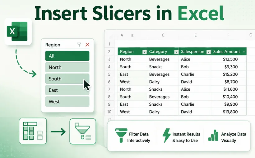
Tired of losing track of your Excel filters inside endless drop-down menus? There's a better way. Slicers turn tedious data exploration into a one‑click visual experience, keeping your selections visible and your dashboards interactive.
In this guide, you'll learn exactly how to insert slicers in Excel, whether you're working with tables or PivotTables. We'll cover best practices for building professional dashboards and even show you how to automate the process with C#.
- What is a Slicer in Excel?
- Why Slicers Outperform Traditional Filters
- Prerequisites Before Inserting Slicers
- How to Add Slicers in Excel: Two Methods
- Advanced: Programmatically Create Slicers in Excel in C#
- How to Use Excel Slicers Once They’re Inserted
- Best Practices for Excel Slicers
- Frequently Asked Questions (FAQs)
What is a Slicer in Excel?
A slicer is a visual filtering tool made up of clickable buttons that correspond to unique values in a data column. Instead of hiding your filter options inside drop-down menus, slicers display them directly on your worksheet, making your current filter state visible at a glance.
Think of slicers as an intuitive control panel for your data. Click a button, and your table, PivotTable, or chart updates instantly. Selected buttons remain highlighted, so you and any other user can always see which filters are active.
Why Slicers Outperform Traditional Filters
| Feature | Traditional Filters | Slicers |
|---|---|---|
| Visibility | Filter state is hidden in drop-down menus | Selected filters are always visible |
| Ease of use | Requires multiple clicks to navigate menu layers | One-click button selection for instant filtering |
| Multi-select | Clunky and unintuitive | Hold Ctrl or use Multi-Select toggle |
| Multiple data sources | Tied to one table | Can control multiple PivotTables and charts |
| Dashboard-friendly | Not designed for dashboards | Perfect for interactive dashboards |
Standard filters force you to click a tiny arrow, uncheck “Select All,” scroll through a long list, and click OK. The moment you click away, your filtering choices disappear from view, leaving you guessing what’s currently applied. Excel slicer tool solves this problem completely by making every filter option a clear, clickable button that sits directly on your worksheet.
Prerequisites Before Inserting Slicers
Before adding slicers in Excel, make sure your data meets these requirements:
- Formatted as Excel Table or PivotTable: Slicers do not work with unformatted raw cell ranges.
- Supported Excel version: Slicers are available in Excel 2013 and later for Windows, and Excel 2016 and later for Mac.
- No blank rows or columns: Empty rows or columns within your dataset can cause Excel to misinterpret the full data range.
- Clean, structured data: Ensure every column has a unique, descriptive header and consistent data formatting.
To convert a range to a table, select your data and press "Ctrl + T", then click OK.
How to Add Slicers in Excel: Two Methods
The process for inserting slicers depends on whether you’re working with a regular Excel Table or a PivotTable. We’ll cover both.
Method 1: Insert Slicers in an Excel Table
- Click anywhere inside your Excel table.
- Go to the Table Design tab on the ribbon.
- Click the Insert Slicer button in the Tools group.

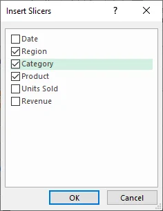
- In the pop-up dialog box, check the boxes for the columns you want to use as slicers (e.g., Region, Product, Category).
- Click OK.
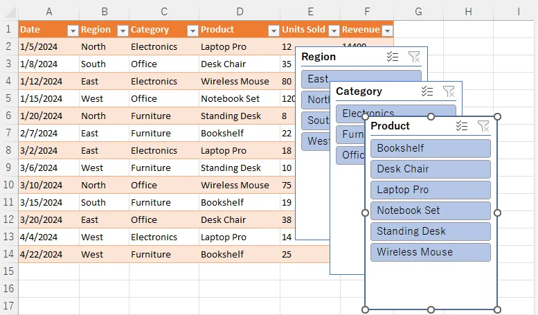
Excel will place slicer objects directly on your worksheet. Each slicer displays buttons for all unique items in its respective field. Click any button inside a slicer to filter the table instantly.
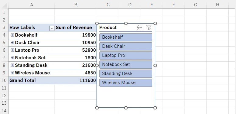
Method 2: Insert Slicers in a PivotTable
- Click any cell inside your pivot table.
- Navigate to the PivotTable Analyze tab (or Analyze tab, depending on your version).
- Click Insert Slicer in the Filter group.

- In the Insert Slicers dialog box, check the boxes for the fields you want to filter by (e.g., Product).
- Click OK.
The slicers appear on your sheet and dynamically update the PivotTable results. You can move, resize, and format them to match your dashboard layout.
Advanced: Programmatically Create Slicers in Excel in C#
While the manual methods are perfect for one‑off tasks, you may need to add slicers to hundreds of Excel files programmatically. That’s where Free Spire.XLS for .NET comes in. This free library allows you to create, read, and modify Excel files without Microsoft Office installed—and it fully supports inserting slicers into Excel tables.
C# Code: Adding Slicers to an Excel Table
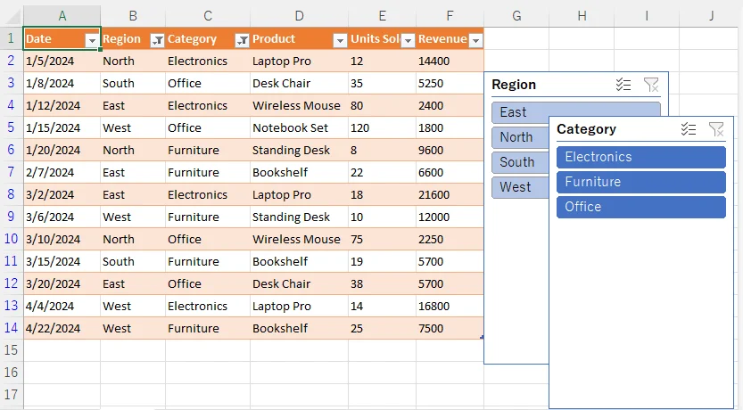
Below is a complete C# example that loads an existing Excel file, retrieves the first table in the first worksheet, and inserts two slicers for two different columns. It then sets a name and a built‑in style for each slicer, and saves the result as a new .xlsx file.
using Spire.Xls;
using Spire.Xls.Core;

namespace AddSlicerToTable
{
    internal class Program
    {
        static void Main(string[] args)
        {
            // Load an Excel file
            Workbook workbook = new Workbook();
            workbook.LoadFromFile("sampleData.xlsx");

            // Get the first worksheet
            Worksheet worksheet = workbook.Worksheets[0];

            // Get the first table in the worksheet
            IListObject table = worksheet.ListObjects[0];

            // Add 2 slicers
            // Parameters: table, location (cell reference), column index (0‑based)
            int slicer1 = worksheet.Slicers.Add(table, "G3", 1);
            int slicer2 = worksheet.Slicers.Add(table, "H5", 2);

            // Set name and style for the slicer
            worksheet.Slicers[slicer1].Name = "Region";
            worksheet.Slicers[slicer1].StyleType = SlicerStyleType.SlicerStyleLight1;
            worksheet.Slicers[slicer2].Name = "Category";
            worksheet.Slicers[slicer2].StyleType = SlicerStyleType.SlicerStyleDark1;

            // Save the result file
            workbook.SaveToFile("AddSlicers.xlsx", ExcelVersion.Version2016);
            workbook.Dispose();
        }
    }
}
How the Slicer API Works
The core method is Slicers.Add() with the following signature:
int Add(IListObject table, string destCellName, int index);
- table: The source IListObject (Excel Table) the slicer is bound to
- destCellName: Top-left cell address where the slicer is placed (e.g., "G3")
- index: 0-based index of the column within the table to use as filter values.
Note: Slicers require a structured Excel Table object. Always create and configure your Excel table first before calling the slicer insertion API.
Result:
Additional Tips for Programmatic Slicer Insertion
- Multiple tables: If your worksheet has more than one table, you can access them via worksheet.ListObjects[index].
-
PivotTable slicers: Free Spire.XLS also supports adding slicers to PivotTables using
worksheet.Slicers.Add(IPivotTable, string, int). -
Saving formats: Use
ExcelVersion.Version2013orVersion2016to ensure slicers are preserved correctly. - Performance: When processing multiple files, create a new Workbook instance for each file and call Dispose() promptly after processing to avoid memory leaks.
How to Use Excel Slicers Once They’re Inserted
Using slicers is remarkably simple:
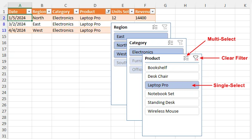
- Single selection: Click any button to filter your data to that value
- Multiple selection: Hold Ctrl as you click multiple buttons, or click the Multi-Select toggle at the top of the slicer panel
- Clear a filter: Click the Clear Filter button (the funnel icon with an X) in the top-right corner of the slicer
Best Practices for Excel Slicers
- Keep slicers grouped and aligned at the top or side of your dashboard.
- Use descriptive captions so viewers understand what each slicer filters.
- Limit the number of slicers — 3–5 usually gives enough interactivity without clutter.
- Name your slicers in the Selection Pane (Alt + F10) for easier management.
- Lock slicer positions (right-click → Size and Properties → Properties → check “Don’t move or size with cells”) so they stay put when users scroll.
- For automation, always target ExcelVersion.Version2016 or higher to ensure slicer compatibility.
Final Thoughts
Adding slicers in Excel is one of the highest-impact skills for anyone building reports or dashboards. For everyday users, they make filtering intuitive, transparent, and dashboard-ready, eliminating the friction of nested drop-down menus. For developers, programmatic slicer APIs enable scalable, automated generation of interactive workbooks at enterprise scale.
Don’t settle for static spreadsheets that confuse your audience. Start using Excel slicers today to unlock the full potential of your data—turning ordinary tables into powerful, interactive decision-making tools that impress and inform.
Frequently Asked Questions (FAQs)
Q: Can I connect one slicer to multiple PivotTables?
A: Yes. Right‑click the slicer → Report Connections → select all PivotTables you want to control.
Q: Can I change slicer colors?
A: Absolutely. Use the Slicer Tools → Options tab to apply built‑in styles or create custom formatting.
Q: Do slicers work with Excel charts?
A: Yes. If a chart is linked to a Table or PivotTable that has an associated slicer, the chart will update automatically to reflect your slicer selections.
Q: Can I change the sort order of items inside a slicer?
A: Yes. Right-click the slicer and select Slicer Settings. In the dialog box, you can choose ascending (A-Z) or descending (Z-A) sort order, or choose to sort using a custom list. You can also control whether items deleted from the source data are retained in the slicer display.