
Knowledgebase (2345)
Children categories
Show formula and its result separately when converting excel to datatable in C#
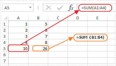
2015-07-10 05:37:43 Written by KoohjiThis article shows how to display formula and its result separately when converting excel to database via Spire.XLS. This demo uses an Excel file with formula in it and show the conversion result in a Windows Forms Application project.
Screenshot of the test excel file:
Here are the detailed steps:
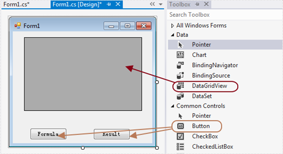
Steps 1: Create a Windows Forms Application in Visual Studio.
Steps 2: Drag a DataGridView and two Buttons from Toolbox to the Form and change names of the buttons as Formula and Result to distinguish.
Steps 3: Double click Button formula and add the following code.
3.1 Load test file and get the first sheet.
Workbook workbook = new Workbook();
workbook.LoadFromFile(@"1.xlsx");
Worksheet sheet = workbook.Worksheets[0];
3.2 Invoke method ExportDataTable of the sheet and output data range. Parameters of ExportDataTable are range to export, indicates if export column name and indicates whether compute formula value, then it will return exported datatable.
Description of ExportDataTable:
public DataTable ExportDataTable(CellRange range, bool exportColumnNames, bool computedFormulaValue);
Code:
DataTable dt = sheet.ExportDataTable(sheet.AllocatedRange, false, false);
3.3 Show in DataGridView
this.dataGridView1.DataSource = dt;
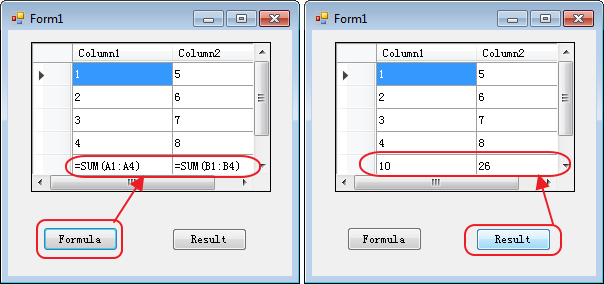
Steps 4: Do ditto to Button Result. Only alter parameter computedFormulaValue as true.
Workbook workbook = new Workbook();
workbook.LoadFromFile(@"1.xlsx");
Worksheet sheet = workbook.Worksheets[0];
DataTable dt = sheet.ExportDataTable(sheet.AllocatedRange, false, true);
this.dataGridView1.DataSource = dt;
Steps 5: Start the project and check the result.
Button code here:
//Formula
private void button1_Click(object sender, EventArgs e)
{
Workbook workbook = new Workbook();
workbook.LoadFromFile(@"1.xlsx");
Worksheet sheet = workbook.Worksheets[0];
DataTable dt = sheet.ExportDataTable(sheet.AllocatedRange, false, false);
this.dataGridView1.DataSource = dt;

}
//Result
private void button2_Click(object sender, EventArgs e)
{
Workbook workbook = new Workbook();
workbook.LoadFromFile(@"1.xlsx");
Worksheet sheet = workbook.Worksheets[0];
DataTable dt = sheet.ExportDataTable(sheet.AllocatedRange, false, true);
this.dataGridView1.DataSource = dt;
}
Gridlines are the faint lines used to distinguish cells in an Excel worksheet. With gridlines, users can easily distinguish the boundaries of each cell and read data in an organized manner. But in certain cases, those gridlines can be quite distracting. In this article, you will learn how to programmatically show or hide/remove gridlines in an Excel worksheet using Spire.XLS for .NET.
Install Spire.XLS for .NET
To begin with, you need to add the DLL files included in the Spire.XLS for .NET package as references in your .NET project. The DLL files can be either downloaded from this link or installed via NuGet.
PM> Install-Package Spire.XLS
Hide or Show Gridlines in Excel
The detailed steps are as follows.
- Create a Workbook object.
- Load a sample Excel document using Workbook.LoadFromFile() method.
- Get a specified worksheet using Workbook.Worksheets[] property.
- Hide or show gridlines in the specified worksheet using Worksheet.GridLinesVisible property.
- Save the result file using Workbook.SaveToFile() method.
- C#
- VB.NET
using Spire.Xls;

namespace RemoveGridlines
{
    class Program
    {

        static void Main(string[] args)
        {
            //Create a Workbook object
            Workbook workbook = new Workbook();

            //Load a sample Excel document
            workbook.LoadFromFile(@"E:\Files\Test.xlsx");

            //Get the first worksheet
            Worksheet worksheet = workbook.Worksheets[0];

            //Hide gridlines in the specified worksheet
            worksheet.GridLinesVisible = false;

            //Show gridlines in the specified worksheet
            //worksheet.GridLinesVisible = true;

            //Save the document
            workbook.SaveToFile("Gridlines.xlsx", ExcelVersion.Version2010);
        }
    }
}
Apply for a Temporary License
If you'd like to remove the evaluation message from the generated documents, or to get rid of the function limitations, please request a 30-day trial license for yourself.
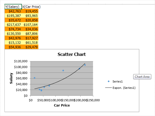
Charts are used to display series of numeric data in a graphical format to make it easier to understand large quantities of data and the relationship between different series of data. This article talks about how to create scatter chart via Spire.XLS.
To create a Scatter Chart, execute the following steps.
Step 1: Create a new Excel document and get the first sheet.
Workbook workbook = new Workbook();
workbook.CreateEmptySheets(1);
Worksheet sheet = workbook.Worksheets[0];
Step 2: Rename the first sheet and set the grid lines invisible.
sheet.Name = "Scatter Chart";
sheet.GridLinesVisible = false;
Step 3: Create a scatter chart and set data region for it.
Chart chart = sheet.Charts.Add(ExcelChartType.ScatterMarkers);
chart.DataRange = sheet.Range["B2:B10"];
chart.SeriesDataFromRange = false;
Step 4: Set position and title for the chart.
chart.LeftColumn = 1;
chart.TopRow = 6;
chart.RightColumn = 9;
chart.BottomRow = 25;

chart.ChartTitle = "Scatter Chart";
chart.ChartTitleArea.IsBold = true;
chart.ChartTitleArea.Size = 12;
Step 5: Add data to the excel range.
sheet.Range["A1"].Value = "Y(Salary)";
sheet.Range["A2"].Value = "42763";
sheet.Range["A3"].Value = "195387";
sheet.Range["A4"].Value = "35672";
sheet.Range["A5"].Value = "217637";
sheet.Range["A6"].Value = "74734";
sheet.Range["A7"].Value = "130550";
sheet.Range["A8"].Value = "42976";
sheet.Range["A9"].Value = "15132";
sheet.Range["A10"].Value = "54936";

sheet.Range["B1"].Value = "X(Car Price)";
sheet.Range["B2"].Value = "19455";
sheet.Range["B3"].Value = "93965";
sheet.Range["B4"].Value = "20858";
sheet.Range["B5"].Value = "107164";
sheet.Range["B6"].Value = "34036";
sheet.Range["B7"].Value = "87806";
sheet.Range["B8"].Value = "17927";
sheet.Range["B9"].Value = "61518";
sheet.Range["B10"].Value = "29479";
Step 6: Set style color for the range.
sheet.Range["A2:B2"].Style.KnownColor = ExcelColors.LightOrange;
sheet.Range["A3:B3"].Style.KnownColor = ExcelColors.LightYellow;
sheet.Range["A4:B4"].Style.KnownColor = ExcelColors.LightOrange;
sheet.Range["A5:B5"].Style.KnownColor = ExcelColors.LightYellow;
sheet.Range["A6:B6"].Style.KnownColor = ExcelColors.LightOrange;
sheet.Range["A7:B7"].Style.KnownColor = ExcelColors.LightYellow;
sheet.Range["A8:B8"].Style.KnownColor = ExcelColors.LightOrange;
sheet.Range["A9:B9"].Style.KnownColor = ExcelColors.LightYellow;
sheet.Range["A10:B10"].Style.KnownColor = ExcelColors.LightOrange;
Step 7: Set number format for cell ranges.
sheet.Range["A2:B10"].Style.NumberFormat = "\"$\"#,##0";
Step 8: Set data for axis x y.
chart.Series[0].CategoryLabels = sheet.Range["A2:A10"];
chart.Series[0].Values = sheet.Range["B2:B10"];
Step 9: Add a trend line.
chart.Series[0].TrendLines.Add(TrendLineType.Exponential);
Step 10: Add axis title.
chart.PrimaryValueAxis.Title = "Salary";
chart.PrimaryCategoryAxis.Title = "Car Price";
Step 11: Save and review.
workbook.SaveToFile("XYChart.xlsx", FileFormat.Version2013);
System.Diagnostics.Process.Start("XYChart.xlsx");
Screenshot:
Full code:
using Spire.Xls;
namespace CreateExcelScatterChart
{
    class Program
    {

        static void Main(string[] args)
        {
            Workbook workbook = new Workbook();
            workbook.CreateEmptySheets(1);
            Worksheet sheet = workbook.Worksheets[0];

            sheet.Name = "Scatter Chart";
            sheet.GridLinesVisible = false;

            Chart chart = sheet.Charts.Add(ExcelChartType.ScatterMarkers);
            chart.DataRange = sheet.Range["B2:B10"];
            chart.SeriesDataFromRange = false;

            chart.LeftColumn = 1;
            chart.TopRow = 6;
            chart.RightColumn = 9;
            chart.BottomRow = 25;

            chart.ChartTitle = "Scatter Chart";
            chart.ChartTitleArea.IsBold = true;
            chart.ChartTitleArea.Size = 12;

            sheet.Range["A1"].Value = "Y(Salary)";
            sheet.Range["A2"].Value = "42763";
            sheet.Range["A3"].Value = "195387";
            sheet.Range["A4"].Value = "35672";
            sheet.Range["A5"].Value = "217637";
            sheet.Range["A6"].Value = "74734";
            sheet.Range["A7"].Value = "130550";
            sheet.Range["A8"].Value = "42976";
            sheet.Range["A9"].Value = "15132";
            sheet.Range["A10"].Value = "54936";

            sheet.Range["B1"].Value = "X(Car Price)";
            sheet.Range["B2"].Value = "19455";
            sheet.Range["B3"].Value = "93965";
            sheet.Range["B4"].Value = "20858";
            sheet.Range["B5"].Value = "107164";
            sheet.Range["B6"].Value = "34036";
            sheet.Range["B7"].Value = "87806";
            sheet.Range["B8"].Value = "17927";
            sheet.Range["B9"].Value = "61518";
            sheet.Range["B10"].Value = "29479";

            sheet.Range["A2:B2"].Style.KnownColor = ExcelColors.LightOrange;
            sheet.Range["A3:B3"].Style.KnownColor = ExcelColors.LightYellow;
            sheet.Range["A4:B4"].Style.KnownColor = ExcelColors.LightOrange;
            sheet.Range["A5:B5"].Style.KnownColor = ExcelColors.LightYellow;
            sheet.Range["A6:B6"].Style.KnownColor = ExcelColors.LightOrange;
            sheet.Range["A7:B7"].Style.KnownColor = ExcelColors.LightYellow;
            sheet.Range["A8:B8"].Style.KnownColor = ExcelColors.LightOrange;
            sheet.Range["A9:B9"].Style.KnownColor = ExcelColors.LightYellow;
            sheet.Range["A10:B10"].Style.KnownColor = ExcelColors.LightOrange;

            sheet.Range["A2:B10"].Style.NumberFormat = "\"$\"#,##0";

            chart.Series[0].CategoryLabels = sheet.Range["A2:A10"];
            chart.Series[0].Values = sheet.Range["B2:B10"];

            chart.Series[0].TrendLines.Add(TrendLineType.Exponential);

            chart.PrimaryValueAxis.Title = "Salary";
            chart.PrimaryCategoryAxis.Title = "Car Price";

            workbook.SaveToFile("XYChart.xlsx", FileFormat.Version2013);
            System.Diagnostics.Process.Start("XYChart.xlsx");
        }
    }
}