
Knowledgebase (2345)
Children categories
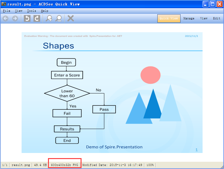
With the help of Spire.Presentation for .NET, we can easily save PowerPoint slides as image in C# and VB.NET. Sometimes, we need to use the resulted images for other purpose and the image size becomes very important. To ensure the image is easy and beautiful to use, we need to set the image with specified size beforehand. This example will demonstrate how to save a particular presentation slide as image with specified size by using Spire.Presentation for your .NET applications.
Note: Before Start, please download the latest version of Spire.Presentation and add Spire.Presentation.dll in the bin folder as the reference of Visual Studio.
Step 1: Create a presentation document and load the document from file.
Presentation presentation = new Presentation();
presentation.LoadFromFile("sample.pptx");
Step 2: Save the first slide to Image and set the image size to 600*400.
Image img = presentation.Slides[0].SaveAsImage(600, 400);
Step 3: Save image to file.
img.Save("result.png",System.Drawing.Imaging.ImageFormat.Png);
Effective screenshot of the resulted image with specified size:
Full codes:
using Spire.Presentation;
using System.Drawing;
namespace SavePowerPointSlideasImage
{
    class Program
    {
        static void Main(string[] args)
        {
            Presentation presentation = new Presentation();
            presentation.LoadFromFile("sample.pptx");

            Image img = presentation.Slides[0].SaveAsImage(600, 400);
            img.Save("result.png", System.Drawing.Imaging.ImageFormat.Png);
        }
    }
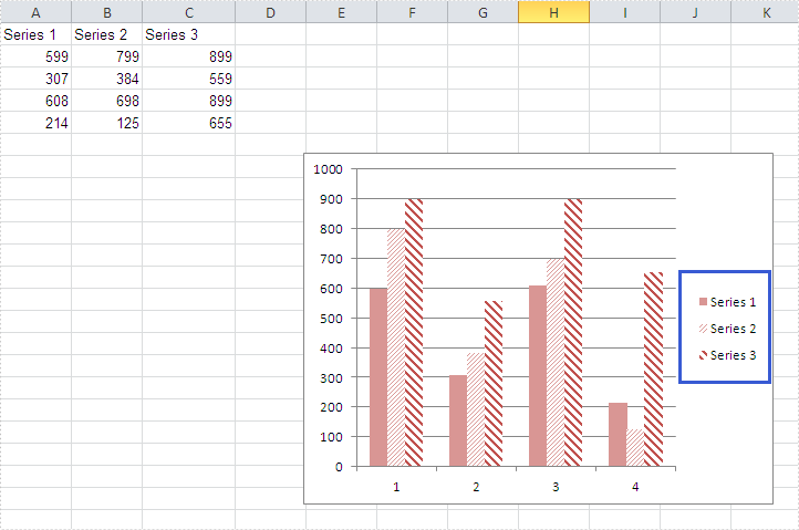
There are many kinds of areas in a chart, such as chart area, plot area, legend area. Spire.XLS offers properties to set the performance of each area easily in C# and VB.NET. We have already shown you how to set the background color and image for chart area and plot area in C#. This article will show you how to set the background color for chart legend in C# with the help of Spire.XLS 7.8.43 or above.
Firstly, please check the original screenshot of excel chart with the automatic setting for chart legend.
Code Snippet of how to set the background color of legend in a Chart:
Step 1: Create a new workbook and load from file.
Workbook workbook = new Workbook();
workbook.LoadFromFile("sample.xlsx");
Step 2: Get the first worksheet from workbook and then get the first chart from the worksheet.
Worksheet ws = workbook.Worksheets[0];
Chart chart = ws.Charts[0];
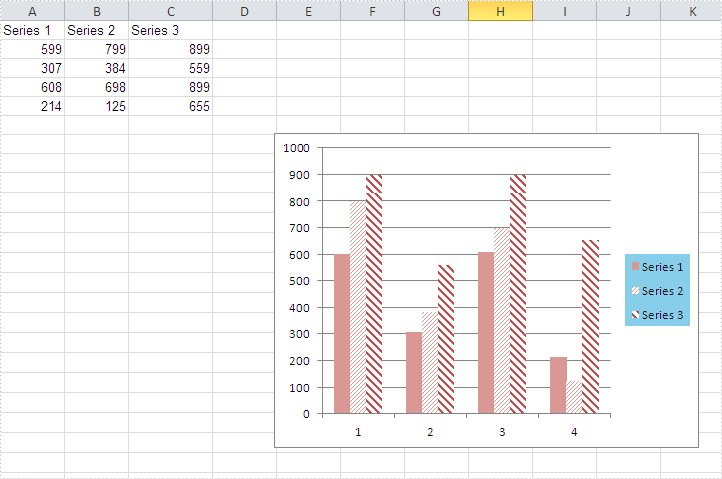
Step 3: Change the background color of the legend in a chart and specify a Solid Fill of SkyBlue.
XlsChartFrameFormat x = chart.Legend.FrameFormat as XlsChartFrameFormat;
x.Fill.FillType = ShapeFillType.SolidColor;
x.ForeGroundColor = Color.SkyBlue;
Step 4: Save the document to file.
workbook.SaveToFile("result.xlsx",ExcelVersion.Version2010);
Effective screenshot after fill the background color for Excel chart legend:
Full codes:
using Spire.Xls;
using Spire.Xls.Core.Spreadsheet.Charts;
using System.Drawing;
namespace SetBackgroundColor
{
    class Program
    {

        static void Main(string[] args)
        {

            Workbook workbook = new Workbook();
            workbook.LoadFromFile("sample.xlsx");

            Worksheet ws = workbook.Worksheets[0];
            Chart chart = ws.Charts[0];

            XlsChartFrameFormat x = chart.Legend.FrameFormat as XlsChartFrameFormat;
            x.Fill.FillType = ShapeFillType.SolidColor;
            x.ForeGroundColor = Color.SkyBlue;

            workbook.SaveToFile("result.xlsx", ExcelVersion.Version2010);
        }
    }
}
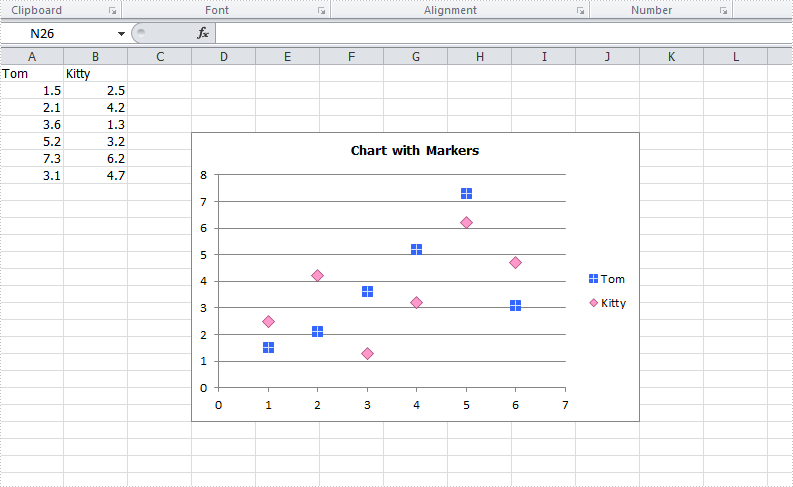
The format of data marker in a line, scatter and radar chart can be changed and customized, which makes it more attractive and distinguishable. We could set markers' built-in type, size, background color, foreground color and transparency in Excel. This article is going to introduce how to achieve those features in C# using Spire.XLS.
Note: before start, please download the latest version of Spire.XLS and add the .dll in the bin folder as the reference of Visual Studio.
Step 1: Create a workbook with sheet and add some sample data.
            Workbook workbook = new Workbook();
            workbook.CreateEmptySheets(1);
            Worksheet sheet = workbook.Worksheets[0];
            sheet.Name = "Demo";
            sheet.Range["A1"].Value = "Tom";
            sheet.Range["A2"].NumberValue = 1.5;
            sheet.Range["A3"].NumberValue = 2.1;
            sheet.Range["A4"].NumberValue = 3.6;
            sheet.Range["A5"].NumberValue = 5.2;
            sheet.Range["A6"].NumberValue = 7.3;
            sheet.Range["A7"].NumberValue = 3.1;
            sheet.Range["B1"].Value = "Kitty";
            sheet.Range["B2"].NumberValue = 2.5;
            sheet.Range["B3"].NumberValue = 4.2;
            sheet.Range["B4"].NumberValue = 1.3;
            sheet.Range["B5"].NumberValue = 3.2;
            sheet.Range["B6"].NumberValue = 6.2;
            sheet.Range["B7"].NumberValue = 4.7;
Step 2: Create a Scatter-Markers chart based on the sample data.
            Chart chart = sheet.Charts.Add(ExcelChartType.ScatterMarkers);
            chart.DataRange = sheet.Range["A1:B7"];
            chart.PlotArea.Visible=false;
            chart.SeriesDataFromRange = false;
            chart.TopRow = 5;
            chart.BottomRow = 22;
            chart.LeftColumn = 4;
            chart.RightColumn = 11;
            chart.ChartTitle = "Chart with Markers";
            chart.ChartTitleArea.IsBold = true;
            chart.ChartTitleArea.Size = 10;
Step 3: Format the markers in the chart by setting the background color, foreground color, type, size and transparency.
            Spire.Xls.Charts.ChartSerie cs1 = chart.Series[0];
            cs1.DataFormat.MarkerBackgroundColor = Color.RoyalBlue;
            cs1.DataFormat.MarkerForegroundColor = Color.WhiteSmoke;
            cs1.DataFormat.MarkerSize = 7;
            cs1.DataFormat.MarkerStyle = ChartMarkerType.PlusSign;
            cs1.DataFormat.MarkerTransparencyValue = 0.8;

            Spire.Xls.Charts.ChartSerie cs2 = chart.Series[1];
            cs2.DataFormat.MarkerBackgroundColor = Color.Pink;
            cs2.DataFormat.MarkerSize = 9;
            cs2.DataFormat.MarkerStyle = ChartMarkerType.Diamond;
            cs2.DataFormat.MarkerTransparencyValue = 0.9;
Step 4: Save the document and launch to see effects.
            workbook.SaveToFile("S3.xlsx", ExcelVersion.Version2010);
            System.Diagnostics.Process.Start("S3.xlsx");
Effects:
Full Codes:
using System;
using System.Collections.Generic;
using System.Linq;
using System.Text;
using Spire.Xls;
using System.Drawing;

namespace ConsoleApplication2
{
    class Program
    {
        static void Main(string[] args)
        {

            Workbook workbook = new Workbook();
            workbook.CreateEmptySheets(1);
            Worksheet sheet = workbook.Worksheets[0];

            sheet.Name = "Demo";
            sheet.Range["A1"].Value = "Tom";
            sheet.Range["A2"].NumberValue = 1.5;
            sheet.Range["A3"].NumberValue = 2.1;
            sheet.Range["A4"].NumberValue = 3.6;
            sheet.Range["A5"].NumberValue = 5.2;
            sheet.Range["A6"].NumberValue = 7.3;
            sheet.Range["A7"].NumberValue = 3.1;
            sheet.Range["B1"].Value = "Kitty";
            sheet.Range["B2"].NumberValue = 2.5;
            sheet.Range["B3"].NumberValue = 4.2;
            sheet.Range["B4"].NumberValue = 1.3;
            sheet.Range["B5"].NumberValue = 3.2;
            sheet.Range["B6"].NumberValue = 6.2;
            sheet.Range["B7"].NumberValue = 4.7;

            Chart chart = sheet.Charts.Add(ExcelChartType.ScatterMarkers);
            chart.DataRange = sheet.Range["A1:B7"];
            chart.PlotArea.Visible=false;
            chart.SeriesDataFromRange = false;
            chart.TopRow = 5;
            chart.BottomRow = 22;
            chart.LeftColumn = 4;
            chart.RightColumn = 11;
            chart.ChartTitle = "Chart with Markers";
            chart.ChartTitleArea.IsBold = true;
            chart.ChartTitleArea.Size = 10;

            Spire.Xls.Charts.ChartSerie cs1 = chart.Series[0];
            cs1.DataFormat.MarkerBackgroundColor = Color.RoyalBlue;
            cs1.DataFormat.MarkerForegroundColor = Color.WhiteSmoke;
            cs1.DataFormat.MarkerSize = 7;
            cs1.DataFormat.MarkerStyle = ChartMarkerType.PlusSign;
            cs1.DataFormat.MarkerTransparencyValue = 0.8;

            Spire.Xls.Charts.ChartSerie cs2 = chart.Series[1];
            cs2.DataFormat.MarkerBackgroundColor = Color.Pink;
            cs2.DataFormat.MarkerSize = 9;
            cs2.DataFormat.MarkerStyle = ChartMarkerType.Diamond;
            cs2.DataFormat.MarkerTransparencyValue = 0.9;

            workbook.SaveToFile("S3.xlsx", ExcelVersion.Version2010);
            System.Diagnostics.Process.Start("S3.xlsx");
        }
    }
}