
Knowledgebase (2345)
Children categories
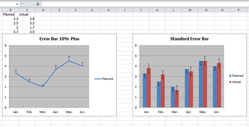
Error bars are a graphical representation of the variability of data and helps us see margins of error and standard deviations immediately in charts with a standard error amount, a percentage, a standard deviation or a custom error amount. Error bars can be used in 2-D area, bar, column, line, scatter, and bubble charts, which are all supported by Spire.XLS. This article is going to introduce the method to add error bars to a chart in C# using Spire.XLS.
Note: before start, please download the latest version of Spire.XLS and add the .dll in the bin folder as the reference of Visual Studio.
Step 1: Create a workbook and fill the sample data in sheet.
            Workbook workbook = new Workbook();
            workbook.CreateEmptySheets(1);
            Worksheet sheet = workbook.Worksheets[0];
            sheet.Name = "Demo";
            sheet.Range["A1"].Value = "Month";
            sheet.Range["A2"].Value = "Jan.";
            sheet.Range["A3"].Value = "Feb.";
            sheet.Range["A4"].Value = "Mar.";
            sheet.Range["A5"].Value = "Apr.";
            sheet.Range["A6"].Value = "May.";
            sheet.Range["A7"].Value = "Jun.";
            sheet.Range["B1"].Value = "Planned";
            sheet.Range["B2"].NumberValue = 3.3;
            sheet.Range["B3"].NumberValue = 2.5;
            sheet.Range["B4"].NumberValue = 2.0;
            sheet.Range["B5"].NumberValue = 3.7;
            sheet.Range["B6"].NumberValue = 4.5;
            sheet.Range["B7"].NumberValue = 4.0;
            sheet.Range["C1"].Value = "Actual";
            sheet.Range["C2"].NumberValue = 3.8;
            sheet.Range["C3"].NumberValue = 3.2;
            sheet.Range["C4"].NumberValue = 1.7;
            sheet.Range["C5"].NumberValue = 3.5;
            sheet.Range["C6"].NumberValue = 4.5;
            sheet.Range["C7"].NumberValue = 4.3;
Step 2: Add a line chart and then add percentage error bar to the chart. The direction of error bars can be set as both, minus and plus and the type of error bars can be set as fixed value, percentage, standard deviation, standard error or custom. After setting the direction and type, we can set the amount.
            Chart chart = sheet.Charts.Add(ExcelChartType.Line);
            chart.DataRange = sheet.Range["B1:B7"];
            chart.SeriesDataFromRange = false;
            chart.TopRow = 6;
            chart.BottomRow = 25;
            chart.LeftColumn = 2;
            chart.RightColumn = 9;
            chart.ChartTitle = "Error Bar 10% Plus";
            chart.ChartTitleArea.IsBold = true;
            chart.ChartTitleArea.Size = 12;
            Spire.Xls.Charts.ChartSerie cs1 = chart.Series[0];
            cs1.CategoryLabels = sheet.Range["A2:A7"];
            cs1.ErrorBar(true, ErrorBarIncludeType.Plus, ErrorBarType.Percentage,10);
Step 3: Add a column chart with standard error bars as comparison.
            Chart chart2 = sheet.Charts.Add(ExcelChartType.ColumnClustered);
            chart2.DataRange = sheet.Range["B1:C7"];
            chart2.SeriesDataFromRange = false;
            chart2.TopRow = 6;
            chart2.BottomRow = 25;
            chart2.LeftColumn = 10;
            chart2.RightColumn = 17;
            chart2.ChartTitle = "Standard Error Bar";
            chart2.ChartTitleArea.IsBold = true;
            chart2.ChartTitleArea.Size = 12;
            Spire.Xls.Charts.ChartSerie cs2 = chart2.Series[0];
            cs2.CategoryLabels = sheet.Range["A2:A7"];
            cs2.ErrorBar(true, ErrorBarIncludeType.Minus, ErrorBarType.StandardError, 0.3);
            Spire.Xls.Charts.ChartSerie cs3 = chart2.Series[1];
            cs3.ErrorBar(true, ErrorBarIncludeType.Both, ErrorBarType.StandardError, 0.5);
Step 4: Save the document and launch to see effects.
            workbook.SaveToFile("S3.xlsx", ExcelVersion.Version2010);
            System.Diagnostics.Process.Start("S3.xlsx");
Effects:
Full Codes:
using System;
using System.Collections.Generic;
using System.Linq;
using System.Text;
using Spire.Xls;
using System.Drawing;

namespace ConsoleApplication2
{
    class Program
    {
        static void Main(string[] args)
        {

            Workbook workbook = new Workbook();
            workbook.CreateEmptySheets(1);
            Worksheet sheet = workbook.Worksheets[0];
            sheet.Name = "Demo";
            sheet.Range["A1"].Value = "Month";
            sheet.Range["A2"].Value = "Jan.";
            sheet.Range["A3"].Value = "Feb.";
            sheet.Range["A4"].Value = "Mar.";
            sheet.Range["A5"].Value = "Apr.";
            sheet.Range["A6"].Value = "May.";
            sheet.Range["A7"].Value = "Jun.";
            sheet.Range["B1"].Value = "Planned";
            sheet.Range["B2"].NumberValue = 3.3;
            sheet.Range["B3"].NumberValue = 2.5;
            sheet.Range["B4"].NumberValue = 2.0;
            sheet.Range["B5"].NumberValue = 3.7;
            sheet.Range["B6"].NumberValue = 4.5;
            sheet.Range["B7"].NumberValue = 4.0;
            sheet.Range["C1"].Value = "Actual";
            sheet.Range["C2"].NumberValue = 3.8;
            sheet.Range["C3"].NumberValue = 3.2;
            sheet.Range["C4"].NumberValue = 1.7;
            sheet.Range["C5"].NumberValue = 3.5;
            sheet.Range["C6"].NumberValue = 4.5;
            sheet.Range["C7"].NumberValue = 4.3;

            Chart chart = sheet.Charts.Add(ExcelChartType.Line);
            chart.DataRange = sheet.Range["B1:B7"];
            chart.SeriesDataFromRange = false;
            chart.TopRow = 6;
            chart.BottomRow = 25;
            chart.LeftColumn = 2;
            chart.RightColumn = 9;
            chart.ChartTitle = "Error Bar 10% Plus";
            chart.ChartTitleArea.IsBold = true;
            chart.ChartTitleArea.Size = 12;
            Spire.Xls.Charts.ChartSerie cs1 = chart.Series[0];
            cs1.CategoryLabels = sheet.Range["A2:A7"];
            cs1.ErrorBar(true, ErrorBarIncludeType.Plus, ErrorBarType.Percentage,10);

            Chart chart2 = sheet.Charts.Add(ExcelChartType.ColumnClustered);
            chart2.DataRange = sheet.Range["B1:C7"];
            chart2.SeriesDataFromRange = false;
            chart2.TopRow = 6;
            chart2.BottomRow = 25;
            chart2.LeftColumn = 10;
            chart2.RightColumn = 17;
            chart2.ChartTitle = "Standard Error Bar";
            chart2.ChartTitleArea.IsBold = true;
            chart2.ChartTitleArea.Size = 12;
            Spire.Xls.Charts.ChartSerie cs2 = chart2.Series[0];
            cs2.CategoryLabels = sheet.Range["A2:A7"];
            cs2.ErrorBar(true, ErrorBarIncludeType.Minus, ErrorBarType.StandardError, 0.3);
            Spire.Xls.Charts.ChartSerie cs3 = chart2.Series[1];
            cs3.ErrorBar(true, ErrorBarIncludeType.Both, ErrorBarType.StandardError, 0.5);

            workbook.SaveToFile("S3.xlsx", ExcelVersion.Version2010);
            System.Diagnostics.Process.Start("S3.xlsx");

        }
    }
}
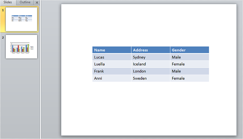
A slide master is the top slide that stores the information about the theme and slide layouts, which will be inherited by other slides in the presentation. In other words, when you modify the style of slide master, every slide in the presentation will be changed accordingly, including the ones added later.
This quality makes it possible that when you want to insert an image or watermark to every slide, you only need to insert the image in slide master. In this article, you'll learn how to add an image to slide master using Spire.Presenation in C#, VB.NET.
Screenshot of original file:
Detailed Steps:
Step 1: Initialize a new Presentation and load the sample file
Presentation presentation = new Presentation();
presentation.LoadFromFile(@"sample.pptx");
Step 2: Get the master collection.
IMasterSlide master = presentation.Masters[0];
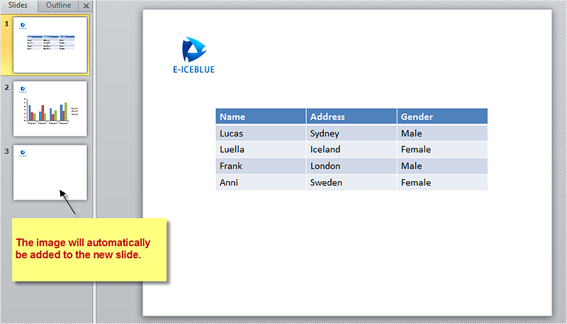
Step 3: Insert an image to slide master.
String image = @"logo.png";
RectangleF rff = new RectangleF(40, 40, 100, 80);
IEmbedImage pic=master.Shapes.AppendEmbedImage(ShapeType.Rectangle, image, rff);
pic.Line.FillFormat.FillType = FillFormatType.None;
Step 4: Add a new blank slide to the presentation.
presentation.Slides.Append();
Step 5: Save and launch the file.
presentation.SaveToFile("result.pptx", FileFormat.Pptx2010);
System.Diagnostics.Process.Start("result.pptx");
Output:
Full Code:
using Spire.Presentation;
using Spire.Presentation.Drawing;
using System;
using System.Drawing;

namespace AddImage
{

    class Program
    {

        static void Main(string[] args)
        {
            //initialize a new Presentation and load the sample file
            Presentation presentation = new Presentation();
            presentation.LoadFromFile(@"sample.pptx");
            //get the master collection
            IMasterSlide master = presentation.Masters[0];
            //append image to slide master
            String image = @"logo.png";
            RectangleF rff = new RectangleF(40, 40, 100, 80);
            IEmbedImage pic = master.Shapes.AppendEmbedImage(ShapeType.Rectangle, image, rff);
            pic.Line.FillFormat.FillType = FillFormatType.None;
            //add new slide to presentation
            presentation.Slides.Append();
            //save and launch the file
            presentation.SaveToFile("result.pptx", FileFormat.Pptx2010);
            System.Diagnostics.Process.Start("result.pptx");
        }
    }
}
Imports Spire.Presentation
Imports Spire.Presentation.Drawing
Imports System.Drawing

Namespace AddImage

	Class Program

		Private Shared Sub Main(args As String())
			'initialize a new Presentation and load the sample file
			Dim presentation As New Presentation()
			presentation.LoadFromFile("sample.pptx")
			'get the master collection
			Dim master As IMasterSlide = presentation.Masters(0)
			'append image to slide master
			Dim image As [String] = "logo.png"
			Dim rff As New RectangleF(40, 40, 100, 80)
			Dim pic As IEmbedImage = master.Shapes.AppendEmbedImage(ShapeType.Rectangle, image, rff)
			pic.Line.FillFormat.FillType = FillFormatType.None
			'add new slide to presentation
			presentation.Slides.Append()
			'save and launch the file
			presentation.SaveToFile("result.pptx", FileFormat.Pptx2010)
			System.Diagnostics.Process.Start("result.pptx")
		End Sub
	End Class
End Namespace
How to format cells with borders in conditional formatting
2015-08-31 01:31:47 Written by AdministratorUsing conditional formatting in Excel, we could highlight interesting cells, emphasize unusual values and visualize data with Data Bars, Color Scales and Icon Sets based on criteria. In the two articles Alternate Row Colors in Excel with Conditional Formatting and Apply Conditional Formatting to a Data Range, we have introduce the method to set fill, font, data bars, color scales and icon sets in conditional formatting using Spire.XLS. This article is going to introduce the method to format cells with borders in conditional formatting.
Note: before start, please download the latest version of Spire.XLS and add the .dll in the bin folder as the reference of Visual Studio.
Step 1: Create a new workbook and add sample data.
            Workbook workbook = new Workbook();
            Worksheet sheet = workbook.Worksheets[0];

            sheet.Range["A1"].Value = "Name/Subject";
            sheet.Range["A2"].Value = "Tom";
            sheet.Range["A3"].Value = "Sam";
            sheet.Range["A4"].Value = "Tina";
            sheet.Range["A5"].Value = "Nancy";
            sheet.Range["A6"].Value = "James";
            sheet.Range["A7"].Value = "Victor";
            sheet.Range["B1"].Value = "Math";
            sheet.Range["C1"].Value = "French";
            sheet.Range["D1"].Value = "English";
            sheet.Range["E1"].Value = "Physics";
            sheet.Range["B2"].NumberValue = 56;
            sheet.Range["B3"].NumberValue = 73;
            sheet.Range["B4"].NumberValue = 75;
            sheet.Range["B5"].NumberValue = 89;
            sheet.Range["B6"].NumberValue = 65;
            sheet.Range["B7"].NumberValue = 90;
            sheet.Range["C2"].NumberValue = 78;
            sheet.Range["C3"].NumberValue = 99;
            sheet.Range["C4"].NumberValue = 86;
            sheet.Range["C5"].NumberValue = 45;
            sheet.Range["C6"].NumberValue = 70;
            sheet.Range["C7"].NumberValue = 83;
            sheet.Range["D2"].NumberValue = 79;
            sheet.Range["D3"].NumberValue = 70;
            sheet.Range["D4"].NumberValue = 90;
            sheet.Range["D5"].NumberValue = 87;
            sheet.Range["D6"].NumberValue = 56;
            sheet.Range["D7"].NumberValue = 78;
            sheet.Range["E2"].NumberValue = 65;
            sheet.Range["E3"].NumberValue = 55;
            sheet.Range["E4"].NumberValue = 100;
            sheet.Range["E5"].NumberValue = 85;
            sheet.Range["E6"].NumberValue = 60;
            sheet.Range["E7"].NumberValue = 75;

            sheet.AllocatedRange.RowHeight = 17;
            sheet.AllocatedRange.ColumnWidth = 17;
            sheet.AllocatedRange.VerticalAlignment = VerticalAlignType.Center;
            sheet.AllocatedRange.HorizontalAlignment = HorizontalAlignType.Center;
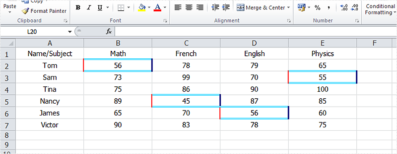
Step 2: Set the formatting rule using formula. Here the rule is the number values less than 60.
XlsConditionalFormats xcfs1 = sheet.ConditionalFormats.Add();
xcfs1.AddRange(sheet.Range["B2:E7"]);
IConditionalFormat format1 = xcfs1.AddCondition();
format1.FormatType = ConditionalFormatType.CellValue;
format1.FirstFormula = "60";
format1.Operator = ComparisonOperatorType.Less;
Step 3: Set border colors and styles for cells that match the condition.
            format1.LeftBorderColor = Color.Red;
            format1.RightBorderColor = Color.DarkBlue;
            format1.TopBorderColor = Color.DeepSkyBlue;
            format1.BottomBorderColor = Color.DeepSkyBlue;

            format1.LeftBorderStyle = LineStyleType.Medium;
            format1.RightBorderStyle = LineStyleType.Thick;
            format1.TopBorderStyle = LineStyleType.Double;
            format1.BottomBorderStyle = LineStyleType.Double;
Step 4: Save the document and launch to see effects.
            workbook.SaveToFile("sample.xlsx", ExcelVersion.Version2010);
            System.Diagnostics.Process.Start("sample.xlsx");
Effects:
Full Codes:
using Spire.Xls;
using Spire.Xls.Core;
using Spire.Xls.Core.Spreadsheet.Collections;
using System.Drawing;

namespace ApplyConditionalFormatting
{
    class Program
    {
        static void Main(string[] args)
        {
            Workbook workbook = new Workbook();
            Worksheet sheet = workbook.Worksheets[0];

            sheet.Range["A1"].Value = "Name/Subject";
            sheet.Range["A2"].Value = "Tom";
            sheet.Range["A3"].Value = "Sam";
            sheet.Range["A4"].Value = "Tina";
            sheet.Range["A5"].Value = "Nancy";
            sheet.Range["A6"].Value = "James";
            sheet.Range["A7"].Value = "Victor";
            sheet.Range["B1"].Value = "Math";
            sheet.Range["C1"].Value = "French";
            sheet.Range["D1"].Value = "English";
            sheet.Range["E1"].Value = "Physics";
            sheet.Range["B2"].NumberValue = 56;
            sheet.Range["B3"].NumberValue = 73;
            sheet.Range["B4"].NumberValue = 75;
            sheet.Range["B5"].NumberValue = 89;
            sheet.Range["B6"].NumberValue = 65;
            sheet.Range["B7"].NumberValue = 90;
            sheet.Range["C2"].NumberValue = 78;
            sheet.Range["C3"].NumberValue = 99;
            sheet.Range["C4"].NumberValue = 86;
            sheet.Range["C5"].NumberValue = 45;
            sheet.Range["C6"].NumberValue = 70;
            sheet.Range["C7"].NumberValue = 83;
            sheet.Range["D2"].NumberValue = 79;
            sheet.Range["D3"].NumberValue = 70;
            sheet.Range["D4"].NumberValue = 90;
            sheet.Range["D5"].NumberValue = 87;
            sheet.Range["D6"].NumberValue = 56;
            sheet.Range["D7"].NumberValue = 78;
            sheet.Range["E2"].NumberValue = 65;
            sheet.Range["E3"].NumberValue = 55;
            sheet.Range["E4"].NumberValue = 100;
            sheet.Range["E5"].NumberValue = 85;
            sheet.Range["E6"].NumberValue = 60;
            sheet.Range["E7"].NumberValue = 75;

            sheet.AllocatedRange.RowHeight = 17;
            sheet.AllocatedRange.ColumnWidth = 17;
            sheet.AllocatedRange.VerticalAlignment = VerticalAlignType.Center;
            sheet.AllocatedRange.HorizontalAlignment = HorizontalAlignType.Center;

            // Apply conditional formatting to the score range (B2:E7)
            XlsConditionalFormats xcfs1 = sheet.ConditionalFormats.Add();
            xcfs1.AddRange(sheet.Range["B2:E7"]);

            // Highlight cells with scores less than 60 using custom borders
            IConditionalFormat format1 = xcfs1.AddCondition();
            format1.FormatType = ConditionalFormatType.CellValue; // Compare cell values
            format1.FirstFormula = "60";
            format1.Operator = ComparisonOperatorType.Less;

            // Set border colors
            format1.LeftBorderColor = Color.Red;
            format1.RightBorderColor = Color.DarkBlue;
            format1.TopBorderColor = Color.DeepSkyBlue;
            format1.BottomBorderColor = Color.DeepSkyBlue;

            // Set border styles
            format1.LeftBorderStyle = LineStyleType.Medium;
            format1.RightBorderStyle = LineStyleType.Thick;
            format1.TopBorderStyle = LineStyleType.Double;
            format1.BottomBorderStyle = LineStyleType.Double;

            workbook.SaveToFile("sample.xlsx", ExcelVersion.Version2010);
            System.Diagnostics.Process.Start("sample.xlsx");
        }
    }
}