Add, Extract or Remove TextBoxes in Excel with JavaScript in React
In daily Excel document processing, textboxes are often used to add explanatory text, annotations, or tips to data — whether adding comments to reports or extracting annotation content from existing documents, the add/remove/modify operations on textboxes are essential. Spire.XLS for JavaScript completes these operations directly in the browser based on WebAssembly, managing input and output files through a virtual file system (VFS), with no backend service required.
This article covers three core features:
For installation and project configuration, refer to Integrating Spire.XLS for JavaScript in a React Project. The examples below assume Spire.XLS is installed and the WebAssembly module is initialized.
Add TextBox
Adding textboxes to a worksheet provides supplementary explanations for data, such as operation guidance or notes. Spire.XLS for JavaScript inserts a textbox at a specified position with the Worksheet.TextBoxes.AddTextBox() method, after which you can set the text, alignment, font, and background color of the textbox, or fill it with a picture. The main steps are as follows:
- Create a
Workbookobject and use theLoadFromFile()method to load the Excel document. - Use the
Workbook.Worksheets.get()method to get a specific worksheet. - Use the
Worksheet.TextBoxes.AddTextBox()method to add the first textbox, and set its text, horizontal/vertical center alignment, font, and background color. - Use the
Worksheet.TextBoxes.AddTextBox()method to add a second textbox and fill it with a picture. - Use the
Workbook.SaveToFile()method to save the document to a specified path.
Here is a complete code example showing how to add two textboxes to a worksheet in React — one containing text and one filled with a picture:
function App() {
  const addTextBox = async () => {
    // Get the Spire.XLS WASM module
    const xlsModule = window.wasmModule?.spirexls;

    // Check whether the module is ready
    if (!xlsModule) {
      alert('Spire.Xls is not ready yet');
      return;
    }

    // Load the font, Excel file and picture into the VFS
    await window.spire.FetchFileToVFS('ARIAL.TTF', '/Library/Fonts/', `${process.env.PUBLIC_URL}/font/`);
    const inputFileName = 'TextBox.xlsx';
    await window.spire.FetchFileToVFS(inputFileName, '', `${process.env.PUBLIC_URL}data/`);
    await window.spire.FetchFileToVFS('logo.png', '', `${process.env.PUBLIC_URL}data/`);

    // Load the workbook
    const workbook = new xlsModule.Workbook();
    workbook.LoadFromFile({ fileName: inputFileName });

    // Get the first worksheet
    const sheet = workbook.Worksheets.get(0);

    // Add the first textbox and set its position and size
    const textBox = sheet.TextBoxes.AddTextBox(3, 2, 50, 196);

    // Set the text in the textbox
    textBox.Text = 'Insert Excel TextBox';

    // Set the text to be centered horizontally and vertically
    textBox.HAlignment = xlsModule.CommentHAlignType.Center;
    textBox.VAlignment = xlsModule.CommentVAlignType.Center;

    // Set the font of the textbox (bold, white, 12pt)
    const font = workbook.CreateFont();
    font.FontName = 'Arial';
    font.Size = 12;
    font.IsBold = true;
    font.Color = xlsModule.Color.get_White();
    const rt = xlsModule.RichTextShape.Convert(textBox.RichText);
    rt.SetFont(0, textBox.Text.length - 1, font);

    // Set the background color of the textbox to blue-gray
    textBox.Fill.FillType = xlsModule.ShapeFillType.SolidColor;
    textBox.Fill.ForeKnownColor = xlsModule.ExcelColors.BlueGray;

    // Add the second textbox and set its position and size
    const textBox2 = sheet.TextBoxes.AddTextBox(6, 5, 90, 90);

    // Load a picture and fill the textbox with it
    textBox2.Fill.CustomPicture('logo.png');
    textBox2.Fill.FillType = xlsModule.ShapeFillType.Picture;

    // Set the border of the second textbox to 0
    textBox2.Line.Weight = 0;

    // Save the document
    const outputFileName = 'AddTextBox_output.xlsx';
    workbook.SaveToFile({ fileName: outputFileName });

    // Release resources
    workbook.Dispose();

    // Read the converted file from the VFS and trigger the download
    const fileArray = window.dotnetRuntime.Module.FS.readFile(outputFileName);
    const blob = new Blob([fileArray], { type: 'application/vnd.openxmlformats-officedocument.spreadsheetml.sheet' });
    const url = URL.createObjectURL(blob);
    const a = document.createElement('a');
    a.href = url;
    a.download = outputFileName;
    a.click();
    URL.revokeObjectURL(url);
  };

  return (
    <div style={{ textAlign: 'center', height: '300px' }}>
      <h1>Add TextBox</h1>
      <button onClick={addTextBox}>
        Start
      </button>
    </div>
  );
}

export default App;
The result of adding the textboxes 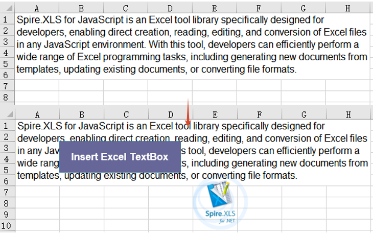
Extract Text and Image from TextBox
When you need to aggregate or reuse annotation information in existing documents, you can iterate through the textboxes and extract their text content and fill images. Spire.XLS for JavaScript gets the number of textboxes with Worksheet.TextBoxes.Count and iterates over each textbox with the Worksheet.TextBoxes.get() method: it reads the Text property to obtain the text content, checks the fill type through Fill.FillType, and extracts the fill image through the Fill.Picture property, finally saving the results as a txt file and a png image file respectively. The main steps are as follows:
- Create a
Workbookobject and use theLoadFromFile()method to load the Excel document. - Use the
Workbook.Worksheets.get()method to get a specific worksheet. - Iterate over each textbox in the
TextBoxescollection withWorksheet.TextBoxes.CountandWorksheet.TextBoxes.get(). - Read the
Textproperty of each textbox to collect the text content. - For a textbox filled with a picture, get its fill image through the
Fill.Pictureproperty and save it as a png file. - Write the collected text into a txt file.
Here is a complete code example showing how to extract text and images from a textbox in React:
function App() {
  const extractTextAndImage = async () => {
    // Get the Spire.XLS WASM module
    const xlsModule = window.wasmModule?.spirexls;

    // Check whether the module is ready
    if (!xlsModule) {
      alert('Spire.Xls is not ready yet');
      return;
    }

    // Load the font and Excel file into the VFS
    await window.spire.FetchFileToVFS('ARIAL.TTF', '/Library/Fonts/', `${process.env.PUBLIC_URL}/font/`);
    const inputFileName = 'TextBox.xlsx';
    await window.spire.FetchFileToVFS(inputFileName, '', `${process.env.PUBLIC_URL}data/`);

    // Load the workbook
    const workbook = new xlsModule.Workbook();
    workbook.LoadFromFile({ fileName: inputFileName });

    // Get the first worksheet
    const sheet = workbook.Worksheets.get(0);

    // Iterate over all textboxes in the worksheet and extract text and pictures
    const textLines = [];
    const pictureFiles = [];
    for (let i = sheet.TextBoxes.Count - 1; i >= 0; i--) {
      const shape = sheet.TextBoxes.get(i);

      // Extract the text in the textbox
      if (shape.Text) {
        textLines.push(shape.Text);
      }

      // Extract the fill picture of the textbox
      if (shape.Fill.FillType === xlsModule.ShapeFillType.Picture) {
        const picture = shape.Fill.Picture;
        const imageFile = 'ExtractedImage' + i + '.png';
        picture.Save(imageFile);
        pictureFiles.push(imageFile);
      }
    }

    // Save the extracted text as a txt file
    const textFile = 'ExtractedText.txt';
    window.dotnetRuntime.Module.FS.writeFile(textFile, textLines.join('\r\n'));

    // Release resources
    workbook.Dispose();

    // Read the extracted txt file from the VFS and trigger the download
    const txtArray = window.dotnetRuntime.Module.FS.readFile(textFile);
    const txtBlob = new Blob([txtArray], { type: 'text/plain' });
    const txtUrl = URL.createObjectURL(txtBlob);
    const txtAnchor = document.createElement('a');
    txtAnchor.href = txtUrl;
    txtAnchor.download = textFile;
    txtAnchor.click();
    URL.revokeObjectURL(txtUrl);

    // Read the extracted picture files from the VFS and trigger the downloads
    for (const imageFile of pictureFiles) {
      const imageArray = window.dotnetRuntime.Module.FS.readFile(imageFile);
      const imageBlob = new Blob([imageArray], { type: 'application/png' });
      const imageUrl = URL.createObjectURL(imageBlob);
      const imageAnchor = document.createElement('a');
      imageAnchor.href = imageUrl;
      imageAnchor.download = imageFile;
      imageAnchor.click();
      URL.revokeObjectURL(imageUrl);
    }
  };

  return (
    <div style={{ textAlign: 'center', height: '300px' }}>
      <h1>Extract Text And Image From TextBox</h1>
      <button onClick={extractTextAndImage}>
        Start
      </button>
    </div>
  );
}

export default App;
The result of extracting the text and image from the textbox 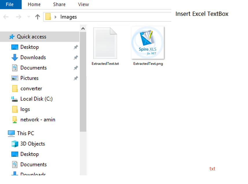
Remove TextBox
When annotation information in a document is no longer needed, you can delete it to keep the worksheet tidy. Spire.XLS for JavaScript deletes a specified textbox by index with the Worksheet.TextBoxes.RemoveAt() method. The main steps are as follows:
- Create a
Workbookobject and use theLoadFromFile()method to load the Excel document. - Use the
Workbook.Worksheets.get()method to get a specific worksheet. - Use the
Worksheet.TextBoxes.RemoveAt()method to delete the textbox at a specified index. - Use the
Workbook.SaveToFile()method to save the document to a specified path.
Here is a complete code example showing how to remove a textbox from a worksheet in React:
function App() {
  const removeTextBox = async () => {
    // Get the Spire.XLS WASM module
    const xlsModule = window.wasmModule?.spirexls;

    // Check whether the module is ready
    if (!xlsModule) {
      alert('Spire.Xls is not ready yet');
      return;
    }

    // Load the font and Excel file into the VFS
    await window.spire.FetchFileToVFS('ARIAL.TTF', '/Library/Fonts/', `${process.env.PUBLIC_URL}/font/`);
    const inputFileName = 'TextBox.xlsx';
    await window.spire.FetchFileToVFS(inputFileName, '', `${process.env.PUBLIC_URL}data/`);

    // Load the workbook
    const workbook = new xlsModule.Workbook();
    workbook.LoadFromFile({ fileName: inputFileName });

    // Get the first worksheet
    const sheet = workbook.Worksheets.get(0);

    // Remove the first textbox
    sheet.TextBoxes.RemoveAt(0);

    // Save the document
    const outputFileName = 'RemoveTextBox_output.xlsx';
    workbook.SaveToFile({ fileName: outputFileName });

    // Release resources
    workbook.Dispose();

    // Read the converted file from the VFS and trigger the download
    const fileArray = window.dotnetRuntime.Module.FS.readFile(outputFileName);
    const blob = new Blob([fileArray], { type: 'application/vnd.openxmlformats-officedocument.spreadsheetml.sheet' });
    const url = URL.createObjectURL(blob);
    const a = document.createElement('a');
    a.href = url;
    a.download = outputFileName;
    a.click();
    URL.revokeObjectURL(url);
  };

  return (
    <div style={{ textAlign: 'center', height: '300px' }}>
      <h1>Remove TextBox</h1>
      <button onClick={removeTextBox}>
        Start
      </button>
    </div>
  );
}

export default App;
The result of removing the textbox 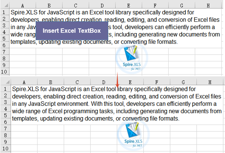
Frequently Asked Questions
The added textbox does not display in the result document
Cause: The row and column coordinates specified in the AddTextBox() method are out of range, or the font file was not loaded into the VFS, so the text in the textbox cannot be rendered properly.
Solution: Make sure the row and column coordinates are within the worksheet range, and ensure the required font has been loaded via FetchFileToVFS() before use, for example:
await window.spire.FetchFileToVFS(
  'ARIAL.TTF', '/Library/Fonts/', '/'
);
An error occurs when extracting an image due to the fill type
Cause: Accessing the Fill.Picture property directly only works for textboxes filled with a picture. If no image fill is set on the textbox (for example, a solid-color fill), accessing this property throws an exception.
Solution: Check whether the Fill.FillType of the textbox is Picture before accessing Fill.Picture; only then get the picture and call the Save() method to save it.
Obtain a Free License
Spire.XLS for JavaScript offers a 30-day full-featured free trial license with no functional limitations. Apply here to evaluate before purchasing.
Insert or Read Functions and Formulas in Excel Worksheets with JavaScript in React
In Excel document processing, formulas and functions are among the most essential capabilities — whether summing, averaging, or performing date and trigonometric operations, formulas make data processing automated and efficient. Spire.XLS for JavaScript completes the insertion and reading of formulas and functions directly in the browser based on WebAssembly, and manages input and output files through a virtual file system (VFS), with no backend service required.
This article covers two core features:
- Insert Formulas and Functions into an Excel Worksheet
- Read Formulas and Functions from an Excel Worksheet
For installation and project configuration, refer to Integrating Spire.XLS for JavaScript in a React Project. The examples below assume Spire.XLS is installed and the WebAssembly module is initialized.
Insert Formulas and Functions into an Excel Worksheet
The Formula property of the cell Range object returned by the Worksheet.Range.get() method in Spire.XLS for JavaScript can be used to add formulas or functions to specified cells in an Excel worksheet. The main steps for adding formulas and functions to an Excel worksheet are as follows:
- Create a
Workbookobject. - Use the
Workbook.Worksheets.get()method to get a specific worksheet. - Write data into cells and set the cell formatting.
- Use the
Range.Formulaproperty to add formulas and functions to the specified cells of the worksheet. - Use the
Workbook.SaveToFile()method to save the workbook.
Here is a complete code example showing how to insert mathematical operations, date functions, trigonometric functions, average functions, and sum functions into an Excel worksheet in React:
function App() {
  const insertFormulasAndFunctions = async () => {
    // Get the Spire.XLS WASM module
    const xlsModule = window.wasmModule?.spirexls;

    // Check whether the module is ready
    if (!xlsModule) {
      alert('Spire.Xls is not ready yet');
      return;
    }

    // Load the font into the VFS
    await window.spire.FetchFileToVFS('ARIAL.TTF', '/Library/Fonts/', `${process.env.PUBLIC_URL}/font/`);

    // Create a Workbook object
    const workbook = new xlsModule.Workbook();

    // Get the first worksheet
    const sheet = workbook.Worksheets.get(0);

    // Declare two variables: currentRow and currentFormula
    let currentRow = 1;
    let currentFormula = "";

    // Set the column width
    sheet.SetColumnWidth(1, 32);
    sheet.SetColumnWidth(2, 16);

    // Write data into cells
    sheet.Range.get({ row: currentRow, column: 1 }).Value = "Test Data";
    sheet.Range.get({ row: currentRow, column: 2 }).NumberValue = 1;
    sheet.Range.get({ row: currentRow, column: 3 }).NumberValue = 2;
    sheet.Range.get({ row: currentRow, column: 4 }).NumberValue = 3;
    sheet.Range.get({ row: currentRow, column: 5 }).NumberValue = 4;
    sheet.Range.get({ row: currentRow, column: 6 }).NumberValue = 5;
    currentRow += 2;
    sheet.Range.get({ row: currentRow, column: 1 }).Value = "Formula or Function";
    sheet.Range.get({ row: currentRow, column: 2 }).Value = "Result";

    // Set the cell formatting
    let range = sheet.Range.get({ row: currentRow, column: 1, lastRow: currentRow, lastColumn: 2 });
    range.Style.Font.FontName = "Arial";
    range.Style.KnownColor = xlsModule.ExcelColors.LightGreen;
    range.Style.FillPattern = xlsModule.ExcelPatternType.Solid;
    range.Style.Borders.get(xlsModule.BordersLineType.EdgeBottom).LineStyle = xlsModule.LineStyleType.Medium;
    range.Style.Font.IsBold = true;

    // Mathematical operation
    currentFormula = "=1/2+3*4";
    currentRow += 1;
    sheet.Range.get({ row: currentRow, column: 1 }).NumberFormat = "@";
    sheet.Range.get({ row: currentRow, column: 1 }).Text = currentFormula;
    sheet.Range.get({ row: currentRow, column: 2 }).Formula = currentFormula;

    // Date function
    currentFormula = "=TODAY()";
    currentRow += 1;
    sheet.Range.get({ row: currentRow, column: 1 }).NumberFormat = "@";
    sheet.Range.get({ row: currentRow, column: 1 }).Text = currentFormula;
    sheet.Range.get({ row: currentRow, column: 2 }).Formula = currentFormula;
    sheet.Range.get({ row: currentRow, column: 2 }).Style.NumberFormat = "YYYY/MM/DD";

    // Trigonometric function
    currentFormula = "=SIN(PI()/6)";
    currentRow += 1;
    sheet.Range.get({ row: currentRow, column: 1 }).NumberFormat = "@";
    sheet.Range.get({ row: currentRow, column: 1 }).Text = currentFormula;
    sheet.Range.get({ row: currentRow, column: 2 }).Formula = currentFormula;

    // Average function
    currentFormula = "=AVERAGE(B1:F1)";
    currentRow += 1;
    sheet.Range.get({ row: currentRow, column: 1 }).NumberFormat = "@";
    sheet.Range.get({ row: currentRow, column: 1 }).Text = currentFormula;
    sheet.Range.get({ row: currentRow, column: 2 }).Formula = currentFormula;

    // Sum function
    currentFormula = "=SUM(B1:F1)";
    currentRow += 1;
    sheet.Range.get({ row: currentRow, column: 1 }).NumberFormat = "@";
    sheet.Range.get({ row: currentRow, column: 1 }).Text = currentFormula;
    sheet.Range.get({ row: currentRow, column: 2 }).Formula = currentFormula;

    // Save the workbook
    const outputFileName = 'InsertFormulasAndFunctions_output.xlsx';
    workbook.SaveToFile({ fileName: outputFileName, version: xlsModule.ExcelVersion.Version2010 });

    // Release resources
    workbook.Dispose();

    // Read the converted file from the VFS and trigger a download
    const fileArray = window.dotnetRuntime.Module.FS.readFile(outputFileName);
    const blob = new Blob([fileArray], { type: 'application/vnd.openxmlformats-officedocument.spreadsheetml.sheet' });
    const url = URL.createObjectURL(blob);
    const a = document.createElement('a');
    a.href = url;
    a.download = outputFileName;
    a.click();
    URL.revokeObjectURL(url);
  };

  return (
    <div style={{ textAlign: 'center', height: '300px' }}>
      <h1>Insert Formulas and Functions</h1>
      <button onClick={insertFormulasAndFunctions}>
        Start
      </button>
    </div>
  );
}

export default App;
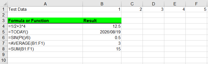
Insert formulas and function results into Excel worksheets
Read Formulas and Functions from an Excel Worksheet
To read formulas and functions from an Excel worksheet, you need to loop through all the used cells in the worksheet, then use the HasFormula property of a cell to find the cells that contain formulas or functions, and finally use the Range.Formula property to get the formulas or functions in those cells. The detailed steps are as follows:
- Create a
Workbookobject. - Use the
Workbook.LoadFromFile()method to load an Excel workbook. - Use the
Workbook.Worksheets.get()method to get the first worksheet. - Loop through the used cells in the worksheet.
- Use the
HasFormulaproperty to detect whether a cell contains a formula or function. If so, use theRange.RangeAddressLocalproperty and theRange.Formulaproperty to get the cell name and its formula or function, and output the retrieved content.
Here is a complete code example showing how to loop through a worksheet and read the formulas and functions in React:
function App() {
  const readFormulasAndFunctions = async () => {
    // Get the Spire.XLS WASM module
    const xlsModule = window.wasmModule?.spirexls;

    // Check whether the module is ready
    if (!xlsModule) {
      alert('Spire.Xls is not ready yet');
      return;
    }

    // Load the font and Excel file into the VFS
    await window.spire.FetchFileToVFS('ARIAL.TTF', '/Library/Fonts/', `${process.env.PUBLIC_URL}/font/`);
    const inputFileName = 'FormulasAndFunctions.xlsx';
    await window.spire.FetchFileToVFS(inputFileName, '', `${process.env.PUBLIC_URL}data/`);

    // Create a Workbook object
    const workbook = new xlsModule.Workbook();

    // Load the Excel workbook
    workbook.LoadFromFile({ fileName: inputFileName });

    // Get the first worksheet
    const sheet = workbook.Worksheets.get(0);

    // Get the used cell range of the worksheet
    const usedRange = sheet.AllocatedRange;

    // Create an output workbook
    const output = new xlsModule.Workbook();
    const outSheet = output.Worksheets.get(0);
    let outRow = 1;

    // Loop through the used cells
    for (const cell of usedRange.Cells) {
      // Check whether the cell contains a formula or function
      if (cell.HasFormula) {
        // Get the cell name
        const cellname = cell.RangeAddressLocal;

        // Get the formula or function in the cell
        const formula = cell.Formula;

        // Write the cell name and formula that were read
        outSheet.Range.get({ row: outRow, column: 1 }).Value = "Cell " + cellname + " contains: " + formula;
        outRow += 1;
      }
    }

    // Set the output column width so the text displays completely
    outSheet.SetColumnWidth(1, 45);

    // Save the output workbook
    const outputFileName = 'ReadFormulasAndFunctions_output.xlsx';
    output.SaveToFile({ fileName: outputFileName, version: xlsModule.ExcelVersion.Version2010 });

    // Release resources
    output.Dispose();

    // Read the converted file from the VFS and trigger a download
    const fileArray = window.dotnetRuntime.Module.FS.readFile(outputFileName);
    const blob = new Blob([fileArray], { type: 'application/vnd.openxmlformats-officedocument.spreadsheetml.sheet' });
    const url = URL.createObjectURL(blob);
    const a = document.createElement('a');
    a.href = url;
    a.download = outputFileName;
    a.click();
    URL.revokeObjectURL(url);
  };

  return (
    <div style={{ textAlign: 'center', height: '300px' }}>
      <h1>Read Formulas and Functions</h1>
      <button onClick={readFormulasAndFunctions}>
        Start
      </button>
    </div>
  );
}

export default App;
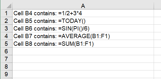
Read formulas and function results from Excel worksheets
Frequently Asked Questions
HasFormula cannot detect the formula, and the loop returns no results
Cause: The formula in the target cell was actually written as text (using the Text/Value property instead of the Formula property), and HasFormula only returns true for real formulas.
Solution: Make sure to use the Range.Formula property when inserting; otherwise, re-assign the text as a formula before reading.
Confusing the Formula and FormulaNumberValue properties
Cause: The Formula property returns the formula string in the cell, while the FormulaNumberValue property returns the numeric result after the formula is calculated. The two return different content.
Solution: Use cell.Formula when you need the formula string, and cell.FormulaNumberValue when you need the numeric result after calculation. Choose the appropriate property based on your actual needs.
Get a Free License
Spire.XLS for JavaScript offers a 30-day full-featured free trial license with no functional limitations. Apply here to evaluate before purchasing.
Group or Ungroup Rows and Columns in Excel with JavaScript in React
In everyday Excel spreadsheet handling, grouping rows or columns lets you collapse detail data and show only summary information, making large tables cleaner and easier to read. Spire.XLS for JavaScript performs grouping and ungrouping directly in the browser based on WebAssembly, and manages input/output files through a virtual file system (VFS), with no backend service required.
This article covers two core features:
For installation and project configuration, refer to Integrate Spire.XLS for JavaScript in a React Project. The examples below assume Spire.XLS is installed and the WebAssembly module is initialized.
Group Rows or Columns
After grouping rows or columns, you can collapse the detail data inside a group and keep only the summary rows or columns you need, making the worksheet tidier. Spire.XLS for JavaScript groups rows with the GroupByRows() method and columns with the GroupByColumns() method. The main steps are as follows:
- Create a
Workbookobject and use theLoadFromFile()method to load the Excel document. - Use the
Workbook.Worksheets.get()method to get a specific worksheet. - Use the
Worksheet.GroupByRows()method to group rows. - Use the
Worksheet.GroupByColumns()method to group columns. - Use the
Workbook.SaveToFile()method to save the document to a specified path.
Here is a complete code example showing how to group rows or columns in React:
function App() {
  const groupRowsAndColumns = async () => {
    // Get the Spire.XLS WASM module
    const xlsModule = window.wasmModule?.spirexls;

    // Check whether the module is ready
    if (!xlsModule) {
      alert('Spire.Xls is not ready yet');
      return;
    }

    // Load the font and Excel file into the VFS
    await window.spire.FetchFileToVFS('ARIAL.TTF', '/Library/Fonts/', `${process.env.PUBLIC_URL}/font/`);
    const inputFileName = 'GroupRowsAndColumns.xlsx';
    await window.spire.FetchFileToVFS(inputFileName, '', `${process.env.PUBLIC_URL}data/`);

    // Load the workbook
    const workbook = new xlsModule.Workbook();
    workbook.LoadFromFile({ fileName: inputFileName });

    // Get the first worksheet
    const sheet = workbook.Worksheets.get(0);

    // Group rows
    sheet.GroupByRows(6, 10, false);
    sheet.GroupByRows(14, 16, false);

    // Group columns
    sheet.GroupByColumns(2, 7, false);

    // Save the document
    const outputFileName = 'GroupRowsAndColumns_output.xlsx';
    workbook.SaveToFile({ fileName: outputFileName, version: xlsModule.ExcelVersion.Version2010 });

    // Release resources
    workbook.Dispose();

    // Read the converted file from the VFS and trigger a download
    const fileArray = window.dotnetRuntime.Module.FS.readFile(outputFileName);
    const blob = new Blob([fileArray], { type: 'application/vnd.openxmlformats-officedocument.spreadsheetml.sheet' });
    const url = URL.createObjectURL(blob);
    const a = document.createElement('a');
    a.href = url;
    a.download = outputFileName;
    a.click();
    URL.revokeObjectURL(url);
  };

  return (
    <div style={{ textAlign: 'center', height: '300px' }}>
      <h1>Group Rows And Columns</h1>
      <button onClick={groupRowsAndColumns}>
        Start
      </button>
    </div>
  );
}

export default App;
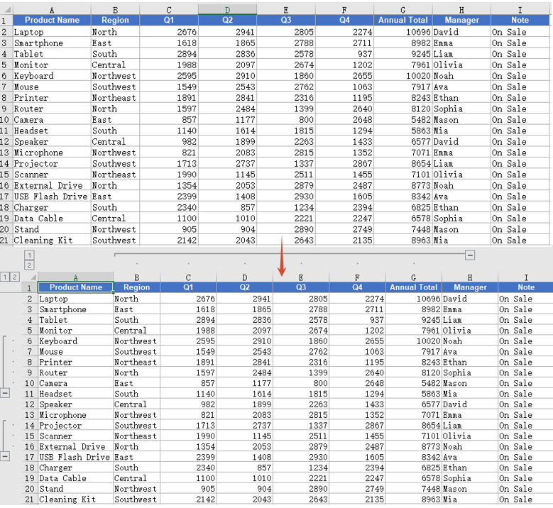
After grouping, group markers appear on the left side of the grouped rows or above the grouped columns. Click a marker to collapse or expand the detail data.
Ungroup Rows or Columns
When the grouping structure is no longer needed, you can ungroup the existing groups so that all rows and columns return to their normal display. Spire.XLS for JavaScript ungroups rows with the UngroupByRows() method and columns with the UngroupByColumns() method. The main steps are as follows:
- Create a
Workbookobject and use theLoadFromFile()method to load the Excel document that contains groups. - Use the
Workbook.Worksheets.get()method to get a specific worksheet. - Use the
Worksheet.UngroupByRows()method to ungroup rows. - Use the
Worksheet.UngroupByColumns()method to ungroup columns. - Use the
Workbook.SaveToFile()method to save the document to a specified path.
Here is a complete code example showing how to ungroup rows or columns in React:
function App() {
  const ungroupRowsAndColumns = async () => {
    // Get the Spire.XLS WASM module
    const xlsModule = window.wasmModule?.spirexls;

    // Check whether the module is ready
    if (!xlsModule) {
      alert('Spire.Xls is not ready yet');
      return;
    }

    // Load the font and Excel file into the VFS
    await window.spire.FetchFileToVFS('ARIAL.TTF', '/Library/Fonts/', `${process.env.PUBLIC_URL}/font/`);
    const inputFileName = 'GroupRowsAndColumns.xlsx';
    await window.spire.FetchFileToVFS(inputFileName, '', `${process.env.PUBLIC_URL}data/`);

    // Load the workbook
    const workbook = new xlsModule.Workbook();
    workbook.LoadFromFile({ fileName: inputFileName });

    // Get the first worksheet
    const sheet = workbook.Worksheets.get(0);

    // Ungroup rows
    sheet.UngroupByRows(6, 10);
    sheet.UngroupByRows(14, 16);

    // Ungroup columns
    sheet.UngroupByColumns(2, 7);

    // Save the document
    const outputFileName = 'UngroupRowsAndColumns_output.xlsx';
    workbook.SaveToFile({ fileName: outputFileName, version: xlsModule.ExcelVersion.Version2010 });

    // Release resources
    workbook.Dispose();

    // Read the converted file from the VFS and trigger a download
    const fileArray = window.dotnetRuntime.Module.FS.readFile(outputFileName);
    const blob = new Blob([fileArray], { type: 'application/vnd.openxmlformats-officedocument.spreadsheetml.sheet' });
    const url = URL.createObjectURL(blob);
    const a = document.createElement('a');
    a.href = url;
    a.download = outputFileName;
    a.click();
    URL.revokeObjectURL(url);
  };

  return (
    <div style={{ textAlign: 'center', height: '300px' }}>
      <h1>Ungroup Rows And Columns</h1>
      <button onClick={ungroupRowsAndColumns}>
        Start
      </button>
    </div>
  );
}

export default App;
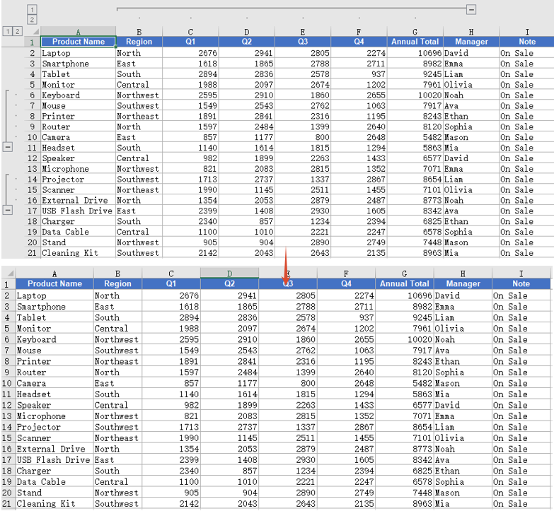
After ungrouping, the group markers on the rows or columns disappear and the data returns to the normal ungrouped display.
FAQ
Cannot collapse or expand detail data after grouping
Cause: The third parameter isCollapsed of the GroupByRows() and GroupByColumns() methods is set to false, so the groups are displayed expanded by default.
Solution: Set this parameter to true, and the groups will be displayed collapsed after saving:
sheet.GroupByRows(6, 10, true);
Some rows or columns still show group symbols after ungrouping
Cause: The UngroupByRows() and UngroupByColumns() methods only ungroup the rows or columns within the specified range. If these rows or columns also belong to a higher-level group, the higher-level group symbols are still retained.
Solution: Make sure the range passed when ungrouping matches the range used when grouping. If nested groups exist, call the ungroup methods repeatedly to ungroup level by level:
sheet.UngroupByRows(6, 10);
sheet.UngroupByRows(14, 16);
sheet.UngroupByColumns(2, 7);
Obtain a Free License
Spire.XLS for JavaScript offers a 30-day full-featured free trial license with no functional limitations. Apply here to evaluate before purchasing.
Como automatizar documentos do Office com um SDK de agente de IA para .NET
Sumário
- A Evolução: De Macros a Agentes de IA
- O Custo Real do Código Orientado a Documentos no .NET
- Arquitetura e APIs Principais do SDK Spire.Agent.Office
- Um Exemplo Prático: Extraindo Dados de Faturas de PDFs
- Além do PDF: Quatro Módulos Especializados de Agentes de IA
- Por que isso é importante para desenvolvedores .NET
- Perguntas Frequentes (FAQs)
Por décadas, a criação de recursos de processamento de documentos seguiu um padrão previsível: lógica de documento mais complexa exigia mais código. Cargas de trabalho comuns, como extrair dados de PDFs, reformatar relatórios do Word ou limpar exportações do Excel, normalmente exigiam centenas de linhas de lógica codificada manualmente, expressões regulares e um tratamento de exceções interminável.
Essa regra está sendo fundamentalmente transformada. Os SDKs de agentes de IA para .NET estão mudando a forma como as empresas lidam com documentos — não tornando o script em C# mais fácil, mas tornando grande parte dele desnecessário.
Conheça o SDK Spire.Agent.Office — um agente de IA para .NET criado especificamente para o ecossistema Office. Com ele, desenvolvedores .NET podem substituir códigos verbosos de travessia e análise por uma única instrução em linguagem natural. Basta descrever o resultado desejado em inglês simples, e o agente o executa para você.
O que você aprenderá neste artigo:
- A Evolução: De Macros a Agentes de IA
- O Custo Real do Código Orientado a Documentos no .NET
- Arquitetura e APIs Principais do SDK Spire.Agent.Office
- Um Exemplo Prático: Extraindo Dados de Faturas de PDFs
- Além do PDF: Quatro Módulos Especializados de Agentes de IA
- Por que isso é importante para desenvolvedores .NET
- Perguntas Frequentes (FAQs)
A Evolução: De Macros a Agentes de IA
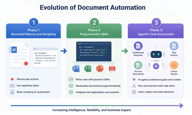
A automação de documentos evoluiu através de fases distintas, cada uma aproximando os desenvolvedores de uma verdadeira interface de programação em linguagem natural.
Fase 1: Macros Gravadas e Scripting
A automação inicial dependia de teclas gravadas e scripts VBA. Essas soluções eram rígidas, quebravam facilmente quando os layouts mudavam e exigiam conhecimento especializado para serem modificadas.
Fase 2: SDKs Programáticos
Bibliotecas como o Spire.Office for .NET deram aos desenvolvedores controle granular sobre os formatos DOCX, XLSX, PPTX e PDF. Embora poderosa, essa abordagem exigia muito código. Uma tarefa simples como "extrair o total de uma fatura" exigia várias linhas de código para lidar com a travessia de páginas, mapeamento de coordenadas e serialização de dados.
Fase 3: Automação de Tarefas com Agentes
Estamos entrando na era dos agentes de IA para documentos. Essas ferramentas não apenas ajudam você a encontrar um método de API específico; elas entendem a intenção de negócio por trás da sua solicitação. Em vez de dizer ao computador como encontrar uma tabela em um documento do Word, você diz a ele o que você quer.
O Custo Real do Código Orientado a Documentos no .NET
A automação tradicional de documentos em C# impõe um fardo pesado aos desenvolvedores:
- Aprender APIs complexas de bibliotecas de documentos especializadas
- Invocar manualmente métodos para carregar arquivos, iterar páginas e analisar conteúdo
- Assumir total responsabilidade pela lógica personalizada de tratamento de erros
O desenvolvedor conduz cada etapa; a biblioteca é meramente uma caixa de ferramentas com funções discretas.
E como um SDK de agente de IA muda isso?
Um SDK de agente de IA para documentos criado para esse fim muda essa dinâmica. Em vez de codificar a lógica de travessia, os usuários definem o resultado de negócio desejado. Com o Spire.Agent.Office, você escreve código C# como este:
// Nova abordagem: uma instrução em linguagem natural
string instruction = "Analise este contrato em busca de cláusulas de risco e gere um resumo.";
AIResult result = processor.ExecuteInstruction(doc, instruction, "resumo.docx");
Nos bastidores, o agente analisa layouts de forma autônoma, extrai conteúdo, executa transformações, valida a saída e se adapta a estruturas inesperadas — tudo sem codificação explícita.
✅ O insight principal: O Spire.Agent.Office possui "capacidade de ação" dentro do domínio de documentos. Ele não sugere apenas trechos de código — ele manipula arquivos diretamente, lê conteúdo, aplica regras de formatação e verifica resultados, tudo controlado por comandos em linguagem natural.
Isso transforma a biblioteca de um kit de ferramentas de codificação em um operador autônomo que conclui tarefas de engenharia de documentos de ponta a ponta em seu nome — enquanto ainda expõe uma superfície de API C# familiar para desenvolvedores .NET.
Arquitetura e APIs Principais do SDK Spire.Agent.Office
A arquitetura é híbrida:
┌─────────────────────────────────────────────────────────────────┐
│  [1]  Camada de Compreensão de IA (LLM configurável)          │
│       • Interpreta instruções em linguagem natural            │
│       • Identifica a intenção de negócio                      │
│       • Planeja as ações necessárias                          │
└─────────────────────────────┬───────────────────────────────────┘
                              │
                              ▼
┌─────────────────────────────────────────────────────────────────┐
│  [2]  Motor de Documento Determinístico (APIs Spire.Office)    │
│       • Executa ações planejadas com precisão                 │
│       • Garante a manipulação precisa de arquivos             │
│       • Assegura layouts perfeitos e formatos corretos        │
└─────────────────────────────────────────────────────────────────┘
Principais componentes do SDK para desenvolvedores .NET:
AIOptions– Classe de configuração para definir seu provedor de IA (OpenAI, Azure, modelos locais, etc.) e chaves de API.AIDocumentProcessor– O ponto de entrada principal, obtido chamando .AI(options) em um objeto de documento (por exemplo, PdfDocument, WordDocument, etc.).ExecuteInstruction()– O método principal que aceita uma instrução em linguagem natural e um caminho de saída opcional, retornando um AIResult contendo status, mensagens e caminhos de arquivos gerados.
Todo o processamento é executado localmente dentro da sua infraestrutura — nenhum conteúdo de documento é enviado para servidores externos, preservando a segurança e a conformidade dos dados — e você pode trocar o LLM subjacente através do AIOptions.
Um Exemplo Prático: Extraindo Dados de Faturas de PDFs
O Desafio: Extrair dados estruturados de faturas em PDF é uma das tarefas mais demoradas para os desenvolvedores.
Abordagem Tradicional
A abordagem programática tradicional exige escrever código para:
- Carregar o PDF e iterar por cada página
- Identificar regiões de texto e limites de tabelas
- Aplicar expressões regulares ou coordenadas posicionais
- Lidar com variações em dezenas de layouts de fornecedores
- Exportar os dados estruturados finais para uma planilha do Excel
Este fluxo de trabalho normalmente exige dezenas de linhas de código C#, preenchidas com lógica posicional frágil e tratamento de exceções para casos extremos.
A Abordagem Spire.Agent.Office
Com o Spire.Agent.Office, um SDK de agente de IA construído sobre o motor de documentos Spire.Office, a mesma tarefa é reduzida a uma única instrução em linguagem natural envolvida em um boilerplate mínimo:
using Spire.Agent.Office.AI;
using Spire.Agent.Office.Extensions;
using Spire.Pdf;

AIOptions options = new AIOptions();
options.SpireToken = "seu-token";

using (PdfDocument pdf = new PdfDocument())
{
    pdf.LoadFromFile("Detalhes_Fatura.pdf");
    AIDocumentProcessor processor = pdf.AI(options);

    string instruction = "Desta tabela de fatura, extraia apenas as linhas onde o Total é maior que $50. " +
                         "Inclua todas as 7 colunas (Item #, Descrição, Qtd, Preço Unitário, Desconto, Preço) e exporte para uma pasta de trabalho do Excel.";

    AIResult result = processor.ExecuteInstruction(
        pdf,
        instruction,
        "dados_fatura_extraidos.xlsx"
    );
}
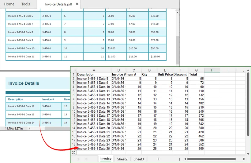
Cerca de 10 linhas de código de suporte + 1 instrução em linguagem natural. Você pode filtrar e exportar as linhas de fatura desejadas para um arquivo Excel.
Visualização do Resultado:
O Fluxo de Trabalho por Trás Disso

Você não precisa mais entender modelos de objetos de documentos, coordenadas de página ou assinaturas de API. Você simplesmente descreve o que deseja na string de instrução.
E quando as regras de negócio evoluem, você atualiza a instrução — não a base de código. Isso reduz drasticamente a sobrecarga de manutenção e acelera os tempos de resposta às necessidades de negócio.
Além do PDF: Quatro Módulos Especializados de Agentes de IA
As capacidades do agente vão muito além do processamento de PDF. O Spire.Agent.Office compreende quatro módulos especializados, cada um adaptado a um formato central de documento do Office, todos controláveis via instruções em linguagem natural:
| Módulo | Tipo de Documento | Capacidades em Linguagem Natural |
|---|---|---|
| Spire.Agent.Doc | Word | Geração de relatórios, revisão de contratos, refinamento de conteúdo, padronização de formato |
| Spire.Agent.XLS | Excel | Relatórios automatizados, limpeza de dados, importação de dados, exportação em múltiplos formatos |
| Spire.Agent.Presentation | PowerPoint | Geração automatizada de slides, atualizações de conteúdo, incorporação de mídia, visualização de dados |
| Spire.Agent.PDF | Operações de mesclagem/divisão, marca d'água, extração de dados, conversão para Word/Excel |
Todos os módulos compartilham o mesmo padrão: configure o AIOptions e, em seguida, faça uma única chamada ExecuteInstruction.
Por que isso é importante para desenvolvedores .NET
Essa evolução não significa o fim para engenheiros de automação ou desenvolvedores .NET. Pelo contrário, ela redefine o trabalho diário deles.
- Menos tempo em E/S de arquivos de baixo nível, mapeamento de coordenadas e boilerplate de tratamento de exceções.
- Mais tempo no design de fluxos de trabalho, regras de validação e integração do agente em processos de negócio maiores.
- Manutenção mais fácil: quando as regras mudam, você atualiza a instrução, não a base de código. Isso reduz o risco de regressão e acelera a resposta às necessidades de negócio.
Os desenvolvedores deixam de ser programadores práticos para se tornarem orquestradores de fluxo de trabalho. Eles definem objetivos de alto nível, supervisionam a saída do agente e tomam decisões estratégicas sobre o que aceitar, refinar ou rejeitar.
Conclusão
Em suma, o Spire.Agent.Office traz capacidades de IA diretamente para seus fluxos de trabalho de documentos. Em vez de escrever centenas de linhas de código complexo para processar arquivos Word, Excel, PowerPoint e PDF, você simplesmente diz ao agente o que precisa em linguagem natural.
Ele lida com o trabalho pesado, incluindo extração de dados, geração de relatórios em lote e formatação de slides, enquanto você mantém controle total sobre a segurança e a precisão. O resultado é um desenvolvimento mais rápido, manutenção mais fácil e mais tempo para focar nos resultados de negócio, não nos detalhes da codificação.
Perguntas Frequentes (FAQs)
P: O Spire.Agent.Office está substituindo a automação de documentos tradicional?
R: Não. Ele a aprimora eliminando a codificação manual para tarefas rotineiras, permitindo que os desenvolvedores foquem em fluxos de trabalho complexos e de alto valor.
P: E quanto à segurança e conformidade?
R: O Spire.Agent.Office opera dentro da sua infraestrutura existente, com todo o processamento ocorrendo localmente. Nenhum conteúdo de documento é enviado externamente.
P: Posso personalizar o comportamento do agente?
R: Sim. Você pode fornecer instruções específicas, definir regras de validação e definir fluxos de trabalho de aprovação para as saídas do agente.
P: Posso trazer meu próprio LLM personalizado ou trocar o modelo de IA subjacente?
R: Sim. O Spire.Agent.Office permite que você configure seus modelos de IA preferidos. Seja OpenAI, Azure OpenAI, um modelo Llama local ou qualquer outro endpoint de IA compatível, você pode conectá-lo à camada de compreensão de IA.
Recursos Adicionais
.NET AI Agent SDK를 사용하여 Office 문서를 자동화하는 방법
수십 년 동안 문서 처리 기능을 구축하는 방식은 예측 가능한 패턴을 따랐습니다. 즉, 문서 로직이 복잡해질수록 더 많은 코드가 필요했습니다. PDF에서 데이터를 추출하거나, Word 보고서의 서식을 다시 지정하거나, Excel 내보내기 파일을 정리하는 등의 일반적인 작업은 보통 수백 줄의 수동 코딩 로직, 정규식, 그리고 끝없는 예외 처리를 필요로 했습니다.
이제 그 규칙이 근본적으로 바뀌고 있습니다. .NET AI 에이전트 SDK는 기업이 문서를 처리하는 방식을 바꾸고 있습니다. C# 스크립팅을 더 쉽게 만드는 것이 아니라, 상당 부분을 불필요하게 만듦으로써 변화를 이끌어냅니다.
Spire.Agent.Office SDK를 소개합니다. 이는 Office 생태계를 위해 특별히 구축된 .NET AI 에이전트입니다. 이를 통해 .NET 개발자는 장황한 탐색 및 파싱 코드를 단 하나의 자연어 지시어로 대체할 수 있습니다. 원하는 결과를 평범한 영어로 설명하기만 하면 에이전트가 대신 실행합니다.
이 기사에서 배우게 될 내용:
- 진화: 매크로에서 AI 에이전트로
- .NET에서 문서 기반 코드의 실제 비용
- Spire.Agent.Office SDK 아키텍처 및 핵심 API
- 실용적인 예제: PDF에서 송장 데이터 추출하기
- PDF를 넘어: 4가지 특화된 AI 에이전트 모듈
- 이것이 .NET 개발자에게 중요한 이유
- 자주 묻는 질문 (FAQs)
진화: 매크로에서 AI 에이전트로
문서 자동화는 뚜렷한 단계를 거쳐 진화해 왔으며, 각 단계는 개발자를 진정한 자연어 프로그래밍 인터페이스에 더 가깝게 만들었습니다.
1단계: 기록된 매크로 및 스크립팅
초기 자동화는 기록된 키 입력과 VBA 스크립트에 의존했습니다. 이러한 솔루션은 경직되어 있었고, 레이아웃이 변경되면 쉽게 깨졌으며, 수정하려면 전문 지식이 필요했습니다.
2단계: 프로그래밍 방식의 SDK
Spire.Office for .NET과 같은 라이브러리는 개발자에게 DOCX, XLSX, PPTX 및 PDF 형식에 대한 세밀한 제어 권한을 제공했습니다. 강력하기는 했지만, 이 방식은 코드 집약적이었습니다. "송장에서 합계 추출"과 같은 간단한 작업도 페이지 탐색, 좌표 매핑, 데이터 직렬화를 처리하기 위해 여러 줄의 코드가 필요했습니다.
3단계: 에이전트 기반 작업 자동화
우리는 이제 문서 AI 에이전트의 시대로 접어들고 있습니다. 이러한 도구는 단순히 특정 API 메서드를 찾는 것을 돕는 데 그치지 않고, 요청 이면의 비즈니스 의도를 이해합니다. Word 문서에서 표를 찾는 방법을 컴퓨터에 지시하는 대신, 무엇을 원하는지만 말하면 됩니다.
.NET에서 문서 기반 코드의 실제 비용
C#에서의 전통적인 문서 자동화는 개발자에게 큰 부담을 줍니다:
- 전문 문서 라이브러리의 복잡한 API 학습
- 파일 로드, 페이지 반복, 콘텐츠 파싱을 위한 메서드 수동 호출
- 사용자 지정 오류 처리 로직에 대한 전적인 책임
개발자가 모든 단계를 주도하며, 라이브러리는 단지 개별 기능의 도구 상자일 뿐입니다.
AI 에이전트 SDK는 이를 어떻게 바꾸는가?
목적에 맞게 구축된 문서 AI 에이전트 SDK는 이러한 역학 관계를 바꿉니다. 탐색 로직을 코딩하는 대신 사용자가 원하는 비즈니스 결과를 정의합니다. Spire.Agent.Office를 사용하면 다음과 같이 C# 코드를 작성할 수 있습니다:
// 새로운 접근 방식: 하나의 자연어 지시어
string instruction = "이 계약서를 검토하여 위험한 조항을 찾고 요약본을 생성하세요.";
AIResult result = processor.ExecuteInstruction(doc, instruction, "summary.docx");
내부적으로 에이전트는 레이아웃을 자율적으로 파싱하고, 콘텐츠를 추출하며, 변환을 실행하고, 출력을 검증하며, 예상치 못한 구조에 적응합니다. 이 모든 과정이 명시적인 코딩 없이 이루어집니다.
✅ 핵심 통찰: Spire.Agent.Office는 문서 도메인 내에서 "실행 능력"을 갖추고 있습니다. 단순히 코드 조각을 제안하는 것이 아니라, 파일을 직접 조작하고, 콘텐츠를 읽고, 서식 규칙을 적용하고, 결과를 검증합니다. 이 모든 것이 자연어 명령을 통해 제어됩니다.
이는 라이브러리를 코딩 툴킷에서 자율 운영자로 변모시켜, .NET 개발자에게 익숙한 C# API 인터페이스를 유지하면서도 엔드 투 엔드 문서 엔지니어링 작업을 대신 수행하게 합니다.
Spire.Agent.Office SDK 아키텍처 및 핵심 API
아키텍처는 하이브리드 형태입니다:
┌─────────────────────────────────────────────────────────────────┐
│  [1]  AI 이해 계층 (구성 가능한 LLM)                           │
│       • 자연어 지시어 해석                                      │
│       • 비즈니스 의도 파악                                      │
│       • 필요한 작업 계획                                        │
└─────────────────────────────┬───────────────────────────────────┘
                              │
                              ▼
┌─────────────────────────────────────────────────────────────────┐
│  [2]  결정론적 문서 엔진 (Spire.Office API)                     │
│       • 계획된 작업을 정밀하게 실행                             │
│       • 정확한 파일 조작 보장                                   │
│       • 픽셀 단위의 완벽한 레이아웃 및 올바른 형식 보장         │
└─────────────────────────────────────────────────────────────────┘
.NET 개발자를 위한 주요 SDK 구성 요소:
AIOptions– AI 공급자(OpenAI, Azure, 로컬 모델 등) 및 API 키를 설정하기 위한 구성 클래스입니다.AIDocumentProcessor– 문서 객체(예: PdfDocument, WordDocument 등)에서 .AI(options)를 호출하여 얻는 주요 진입점입니다.ExecuteInstruction()– 자연어 지시어와 선택적 출력 경로를 받아 상태, 메시지, 생성된 파일 경로가 포함된 AIResult를 반환하는 핵심 메서드입니다.
모든 처리는 인프라 내에서 로컬로 실행되므로 문서 콘텐츠가 외부 서버로 전송되지 않아 데이터 보안과 규정 준수를 유지할 수 있으며, AIOptions를 통해 기본 LLM을 교체할 수 있습니다.
실용적인 예제: PDF에서 송장 데이터 추출하기
과제: PDF 송장에서 구조화된 데이터를 추출하는 것은 개발자에게 가장 시간이 많이 걸리는 작업 중 하나입니다.
전통적인 접근 방식
전통적인 프로그래밍 방식은 다음을 수행하는 코드를 작성해야 합니다:
- PDF를 로드하고 모든 페이지를 반복
- 텍스트 영역 및 표 경계 식별
- 정규식 또는 위치 좌표 적용
- 수십 개의 공급업체 레이아웃에 따른 변형 처리
- 최종 구조화된 데이터를 Excel 시트로 내보내기
이 워크플로우는 일반적으로 수십 줄의 C# 코드를 필요로 하며, 취약한 위치 기반 로직과 예외 처리로 가득 차 있습니다.
Spire.Agent.Office 접근 방식
성숙한 Spire.Office 문서 엔진을 기반으로 구축된 AI 에이전트 SDK인 Spire.Agent.Office를 사용하면 동일한 작업을 최소한의 상용구 코드로 감싼 단 하나의 자연어 지시어로 줄일 수 있습니다:
using Spire.Agent.Office.AI;
using Spire.Agent.Office.Extensions;
using Spire.Pdf;

AIOptions options = new AIOptions();
options.SpireToken = "your-token";

using (PdfDocument pdf = new PdfDocument())
{
    pdf.LoadFromFile("Invoice Details.pdf");
    AIDocumentProcessor processor = pdf.AI(options);

    string instruction = "이 송장 표에서 합계가 $50보다 큰 행만 추출하세요. " +
                         "7개 열(항목 번호, 설명, 수량, 단가, 할인, 가격)을 모두 포함하여 Excel 통합 문서로 내보내세요.";

    AIResult result = processor.ExecuteInstruction(
        pdf,
        instruction,
        "extracted_invoice_data.xlsx"
    );
}
약 10줄의 지원 코드 + 1개의 자연어 지시어. 대상 송장 행을 필터링하여 Excel 파일로 내보낼 수 있습니다.
결과 미리보기:
그 이면의 워크플로우
더 이상 문서 객체 모델, 페이지 좌표 또는 API 시그니처를 이해할 필요가 없습니다. 지시어 문자열에 원하는 내용을 설명하기만 하면 됩니다.
비즈니스 규칙이 변경되면 코드베이스가 아닌 지시어만 업데이트하면 됩니다. 이는 유지 관리 오버헤드를 획기적으로 줄이고 비즈니스 요구에 대한 대응 속도를 높입니다.
PDF를 넘어: 4가지 특화된 AI 에이전트 모듈
에이전트의 기능은 PDF 처리를 훨씬 뛰어넘습니다. Spire.Agent.Office는 4개의 특화된 모듈로 구성되어 있으며, 각 모듈은 핵심 Office 문서 형식에 맞춰져 있고 모두 자연어 지시어를 통해 제어할 수 있습니다:
| 모듈 | 문서 유형 | 자연어 기능 |
|---|---|---|
| Spire.Agent.Doc | Word | 보고서 생성, 계약서 검토, 콘텐츠 개선, 형식 표준화 |
| Spire.Agent.XLS | Excel | 자동 보고, 데이터 정리, 데이터 가져오기, 다중 형식 내보내기 |
| Spire.Agent.Presentation | PowerPoint | 자동 슬라이드 생성, 콘텐츠 업데이트, 미디어 삽입, 데이터 시각화 |
| Spire.Agent.PDF | 병합/분할 작업, 워터마킹, 데이터 추출, Word/Excel로 변환 |
모든 모듈은 동일한 패턴을 공유합니다: AIOptions를 구성한 다음 ExecuteInstruction을 한 번 호출하면 됩니다.
이것이 .NET 개발자에게 중요한 이유
이러한 진화가 자동화 엔지니어나 .NET 개발자의 끝을 의미하는 것은 아닙니다. 오히려 그들의 일상 업무를 재정의합니다.
- 저수준 파일 I/O, 좌표 매핑 및 예외 처리 상용구 코드에 소요되는 시간 단축.
- 워크플로우 설계, 유효성 검사 규칙, 에이전트를 더 큰 비즈니스 프로세스에 통합하는 데 더 많은 시간 할애.
- 더 쉬운 유지 관리: 규칙이 변경되면 코드베이스가 아닌 지시어를 업데이트합니다. 이는 회귀 위험을 줄이고 비즈니스 요구에 대한 대응 속도를 높입니다.
개발자는 직접 스크립트를 작성하는 사람에서 워크플로우 오케스트레이터로 전환됩니다. 그들은 상위 수준의 목표를 정의하고, 에이전트의 출력을 감독하며, 무엇을 수락, 개선 또는 거부할지에 대한 전략적 결정을 내립니다.
결론
요약하자면, Spire.Agent.Office는 AI 기능을 문서 워크플로우에 직접 도입합니다. Word, Excel, PowerPoint 및 PDF 파일을 처리하기 위해 수백 줄의 복잡한 코드를 작성하는 대신, 자연어로 필요한 내용을 에이전트에게 말하기만 하면 됩니다.
데이터 추출, 배치 보고서 생성 및 슬라이드 서식 지정을 포함한 고강도 작업을 에이전트가 처리하는 동안, 사용자는 보안과 정확성에 대한 완전한 통제권을 유지합니다. 그 결과 개발 속도가 빨라지고 유지 관리가 쉬워지며, 코딩 세부 사항이 아닌 비즈니스 결과에 집중할 수 있는 시간이 늘어납니다.
자주 묻는 질문 (FAQs)
Q: Spire.Agent.Office가 기존 문서 자동화를 대체하나요?
A: 아니요. 일상적인 작업에 대한 수동 코딩을 제거하여 자동화를 향상시키는 동시에, 개발자가 복잡하고 가치 높은 워크플로우에 집중할 수 있도록 합니다.
Q: 보안 및 규정 준수는 어떻게 되나요?
A: Spire.Agent.Office는 기존 인프라 내에서 작동하며 모든 처리가 로컬에서 수행됩니다. 문서 콘텐츠는 외부로 전송되지 않습니다.
Q: 에이전트의 동작을 사용자 지정할 수 있나요?
A: 네. 특정 지시어를 제공하고, 유효성 검사 규칙을 설정하며, 에이전트 출력에 대한 승인 워크플로우를 정의할 수 있습니다.
Q: 나만의 맞춤형 LLM을 가져오거나 기본 AI 모델을 전환할 수 있나요?
A: 네. Spire.Agent.Office를 사용하면 선호하는 AI 모델을 설정할 수 있습니다. OpenAI, Azure OpenAI, 로컬 Llama 모델 또는 기타 호환 가능한 AI 엔드포인트 등 무엇이든 AI 이해 계층에 연결할 수 있습니다.
추가 리소스
Come automatizzare i documenti Office con un SDK per agenti IA .NET
Indice
- L'evoluzione: dalle macro agli agenti AI
- Il costo reale del codice basato su documenti in .NET
- Architettura e API principali dell'SDK Spire.Agent.Office
- Un esempio pratico: estrazione di dati di fatturazione da PDF
- Oltre il PDF: quattro moduli di agenti AI specializzati
- Perché è importante per gli sviluppatori .NET
- Domande frequenti (FAQ)
Per decenni, la creazione di funzionalità di elaborazione documenti ha seguito uno schema prevedibile: una logica documentale più complessa richiedeva più codice. Carichi di lavoro comuni come l'estrazione di dati da PDF, la riformattazione di report Word o la pulizia di esportazioni Excel richiedevano solitamente centinaia di righe di logica scritta a mano, espressioni regolari e una gestione infinita delle eccezioni.
Questa regola sta ora subendo una trasformazione fondamentale. Gli SDK di agenti AI per .NET stanno cambiando il modo in cui le aziende gestiscono i documenti, non rendendo più semplice lo scripting in C#, ma rendendo gran parte di esso non necessario.
Ti presentiamo Spire.Agent.Office SDK: un agente AI per .NET creato specificamente per l'ecosistema Office. Con esso, gli sviluppatori .NET possono sostituire il codice prolisso di attraversamento e parsing con una singola istruzione in linguaggio naturale. Descrivi semplicemente il risultato desiderato in un inglese semplice e l'agente lo eseguirà per te.
Cosa imparerai in questo articolo:
- L'evoluzione: dalle macro agli agenti AI
- Il costo reale del codice basato su documenti in .NET
- Architettura e API principali dell'SDK Spire.Agent.Office
- Un esempio pratico: estrazione di dati di fatturazione da PDF
- Oltre il PDF: quattro moduli di agenti AI specializzati
- Perché è importante per gli sviluppatori .NET
- Domande frequenti (FAQ)
L'evoluzione: dalle macro agli agenti AI
L'automazione dei documenti si è evoluta attraverso fasi distinte, ognuna delle quali ha avvicinato gli sviluppatori a una vera interfaccia di programmazione in linguaggio naturale.
Fase 1: Macro registrate e scripting
L'automazione iniziale si basava su sequenze di tasti registrate e script VBA. Queste soluzioni erano rigide, si rompevano facilmente al cambiare dei layout e richiedevano conoscenze specialistiche per essere modificate.
Fase 2: SDK programmatici
Librerie come Spire.Office for .NET hanno fornito agli sviluppatori un controllo granulare sui formati DOCX, XLSX, PPTX e PDF. Sebbene potente, questo approccio richiedeva molto codice. Un compito semplice come "estrarre il totale da una fattura" richiedeva molteplici righe di codice per gestire l'attraversamento delle pagine, la mappatura delle coordinate e la serializzazione dei dati.
Fase 3: Automazione dei compiti tramite agenti
Stiamo entrando nell'era degli agenti AI per documenti. Questi strumenti non ti aiutano solo a trovare un metodo API specifico; comprendono l'intento aziendale dietro la tua richiesta. Invece di dire al computer come trovare una tabella in un documento Word, gli dici cosa vuoi.
Il costo reale del codice basato su documenti in .NET
L'automazione documentale tradizionale in C# pone un pesante fardello sugli sviluppatori:
- Apprendere API complesse da librerie documentali specializzate
- Invocare manualmente metodi per caricare file, scorrere pagine e analizzare contenuti
- Assumersi la piena responsabilità della logica di gestione degli errori personalizzata
Lo sviluppatore guida ogni passaggio; la libreria è semplicemente una cassetta degli attrezzi di funzioni discrete.
E come lo cambia un SDK di agenti AI?
Un SDK di agenti AI per documenti appositamente progettato cambia questa dinamica. Invece di scrivere la logica di attraversamento, gli utenti definiscono il risultato aziendale desiderato. Con Spire.Agent.Office, scrivi codice C# come questo:
// Nuovo approccio: un'istruzione in linguaggio naturale
string instruction = "Esamina questo contratto per clausole rischiose e genera un riepilogo.";
AIResult result = processor.ExecuteInstruction(doc, instruction, "riepilogo.docx");
Dietro le quinte, l'agente analizza autonomamente i layout, estrae contenuti, esegue trasformazioni, convalida l'output e si adatta a strutture impreviste, il tutto senza codifica esplicita.
✅ L'intuizione principale: Spire.Agent.Office possiede una "capacità di azione" all'interno del dominio documentale. Non suggerisce semplicemente frammenti di codice: manipola direttamente i file, legge i contenuti, applica regole di formattazione e verifica i risultati, il tutto controllato tramite comandi in linguaggio naturale.
Questo trasforma la libreria da un toolkit di codifica a un operatore autonomo che completa attività di ingegneria documentale end-to-end per tuo conto, pur esponendo una familiare superficie API C# per gli sviluppatori .NET.
Architettura e API principali dell'SDK Spire.Agent.Office
L'architettura è ibrida:
┌─────────────────────────────────────────────────────────────────┐
│  [1]  Livello di comprensione AI (LLM configurabile)          │
│       • Interpreta le istruzioni in linguaggio naturale       │
│       • Identifica l'intento aziendale                        │
│       • Pianifica le azioni necessarie                        │
└─────────────────────────────┬───────────────────────────────────┘
                              │
                              ▼
┌─────────────────────────────────────────────────────────────────┐
│  [2]  Motore documentale deterministico (API Spire.Office)    │
│       • Esegue le azioni pianificate con precisione           │
│       • Garantisce una manipolazione accurata dei file        │
│       • Assicura layout perfetti e formati corretti           │
└─────────────────────────────────────────────────────────────────┘
Componenti chiave dell'SDK per sviluppatori .NET:
AIOptions: classe di configurazione per impostare il tuo provider AI (OpenAI, Azure, modelli locali, ecc.) e le chiavi API.AIDocumentProcessor: il punto di ingresso principale, ottenuto chiamando .AI(options) su un oggetto documento (ad esempio, PdfDocument, WordDocument, ecc.).ExecuteInstruction(): il metodo principale che accetta un'istruzione in linguaggio naturale e un percorso di output opzionale, restituendo un AIResult contenente stato, messaggi e percorsi dei file generati.
Tutta l'elaborazione viene eseguita localmente all'interno della tua infrastruttura: nessun contenuto del documento viene inviato a server esterni, preservando la sicurezza dei dati e la conformità. Inoltre, puoi sostituire l'LLM sottostante tramite AIOptions.
Un esempio pratico: estrazione di dati di fatturazione da PDF
La sfida: l'estrazione di dati strutturati da fatture PDF è uno dei compiti più dispendiosi in termini di tempo per gli sviluppatori.
Approccio tradizionale
L'approccio programmatico tradizionale richiede la scrittura di codice per:
- Caricare il PDF e scorrere ogni pagina
- Identificare le regioni di testo e i confini delle tabelle
- Applicare espressioni regolari o coordinate posizionali
- Gestire le variazioni tra decine di layout dei fornitori
- Esportare i dati strutturati finali in un foglio Excel
Questo flusso di lavoro richiede solitamente decine di righe di codice C#, piene di logica posizionale fragile e gestione delle eccezioni per casi limite.
L'approccio Spire.Agent.Office
Con Spire.Agent.Office, un SDK di agenti AI costruito sul maturo motore documentale Spire.Office, lo stesso compito è ridotto a una singola istruzione in linguaggio naturale racchiusa in un boilerplate minimo:
using Spire.Agent.Office.AI;
using Spire.Agent.Office.Extensions;
using Spire.Pdf;

AIOptions options = new AIOptions();
options.SpireToken = "il-tuo-token";

using (PdfDocument pdf = new PdfDocument())
{
    pdf.LoadFromFile("Dettagli Fattura.pdf");
    AIDocumentProcessor processor = pdf.AI(options);

    string instruction = "Da questa tabella di fatturazione, estrai solo le righe in cui il Totale è superiore a 50$. " +
                         "Includi tutte e 7 le colonne (N. Articolo, Descrizione, Qtà, Prezzo Unitario, Sconto, Prezzo) ed esporta in una cartella di lavoro Excel.";

    AIResult result = processor.ExecuteInstruction(
        pdf,
        instruction,
        "dati_fattura_estratti.xlsx"
    );
}
Circa 10 righe di codice di supporto + 1 istruzione in linguaggio naturale. Puoi filtrare ed esportare le righe della fattura target in un file Excel.
Anteprima del risultato:
Il flusso di lavoro dietro di esso
Non hai più bisogno di comprendere modelli a oggetti documentali, coordinate di pagina o firme API. Descrivi semplicemente ciò che vuoi nella stringa di istruzione.
E quando le regole aziendali si evolvono, aggiorni l'istruzione, non la base di codice. Ciò riduce drasticamente i costi di manutenzione e accelera i tempi di risposta alle esigenze aziendali.
Oltre il PDF: quattro moduli di agenti AI specializzati
Le capacità dell'agente si estendono ben oltre l'elaborazione PDF. Spire.Agent.Office comprende quattro moduli specializzati, ognuno adattato a un formato di documento Office principale, tutti controllabili tramite istruzioni in linguaggio naturale:
| Modulo | Tipo di documento | Capacità in linguaggio naturale |
|---|---|---|
| Spire.Agent.Doc | Word | Generazione di report, revisione contratti, perfezionamento dei contenuti, standardizzazione del formato |
| Spire.Agent.XLS | Excel | Reportistica automatizzata, pulizia dei dati, importazione dati, esportazione multiformato |
| Spire.Agent.Presentation | PowerPoint | Generazione automatizzata di slide, aggiornamenti dei contenuti, incorporamento di media, visualizzazione dati |
| Spire.Agent.PDF | Operazioni di unione/divisione, filigrana, estrazione dati, conversione in Word/Excel |
Tutti i moduli condividono lo stesso schema: configura AIOptions, quindi effettua una singola chiamata ExecuteInstruction.
Perché è importante per gli sviluppatori .NET
Questa evoluzione non segna la fine per gli ingegneri dell'automazione o gli sviluppatori .NET. Piuttosto, ridefinisce il loro lavoro quotidiano.
- Meno tempo su I/O di file di basso livello, mappatura delle coordinate e boilerplate di gestione delle eccezioni.
- Più tempo sulla progettazione del flusso di lavoro, sulle regole di convalida e sull'integrazione dell'agente in processi aziendali più ampi.
- Manutenzione più semplice: quando le regole cambiano, aggiorni l'istruzione, non la base di codice. Ciò riduce il rischio di regressione e accelera la risposta alle esigenze aziendali.
Gli sviluppatori passano dall'essere scripter pratici a orchestratori di flussi di lavoro. Definiscono obiettivi di alto livello, supervisionano l'output dell'agente e prendono decisioni strategiche su cosa accettare, perfezionare o rifiutare.
Conclusione
In breve, Spire.Agent.Office porta le capacità dell'AI direttamente nei tuoi flussi di lavoro documentali. Invece di scrivere centinaia di righe di codice complesso per elaborare file Word, Excel, PowerPoint e PDF, dici semplicemente all'agente ciò di cui hai bisogno in linguaggio naturale.
Gestisce il lavoro pesante, inclusa l'estrazione dei dati, la generazione di report in batch e la formattazione delle slide, mentre tu mantieni il pieno controllo della sicurezza e dell'accuratezza. Il risultato è uno sviluppo più rapido, una manutenzione più semplice e più tempo per concentrarsi sui risultati aziendali, non sui dettagli della codifica.
Domande frequenti (FAQ)
D: Spire.Agent.Office sostituirà l'automazione documentale tradizionale?
R: No. La migliora eliminando la codifica manuale per le attività di routine, consentendo al contempo agli sviluppatori di concentrarsi su flussi di lavoro complessi e ad alto valore.
D: Che dire della sicurezza e della conformità?
R: Spire.Agent.Office opera all'interno della tua infrastruttura esistente, con tutta l'elaborazione che avviene localmente. Nessun contenuto del documento viene inviato esternamente.
D: Posso personalizzare il comportamento dell'agente?
R: Sì. Puoi fornire istruzioni specifiche, impostare regole di convalida e definire flussi di lavoro di approvazione per gli output dell'agente.
D: Posso utilizzare il mio LLM personalizzato o cambiare il modello AI sottostante?
R: Sì. Spire.Agent.Office ti consente di impostare i tuoi modelli AI preferiti. Che si tratti di OpenAI, Azure OpenAI, un modello Llama locale o qualsiasi altro endpoint AI compatibile, puoi collegarlo al livello di comprensione AI.
Risorse aggiuntive
Comment automatiser les documents Office avec un SDK d'agent IA .NET
Table des matières
- L'évolution : des macros aux agents IA
- Le coût réel du code basé sur les documents en .NET
- Architecture et API principales du SDK Spire.Agent.Office
- Exemple pratique : extraction de données de factures à partir d'un PDF
- Au-delà du PDF : quatre modules d'agents IA spécialisés
- Pourquoi est-ce important pour les développeurs .NET ?
- Foire aux questions (FAQ)
Pendant des décennies, la création de fonctionnalités de traitement de documents a suivi un schéma prévisible : une logique documentaire plus complexe exigeait plus de code. Les tâches courantes telles que l'extraction de données à partir de PDF, le reformatage de rapports Word ou le nettoyage d'exportations Excel nécessitaient généralement des centaines de lignes de logique codée manuellement, des expressions régulières et une gestion interminable des exceptions.
Cette règle est désormais fondamentalement transformée. Les SDK d'agents IA pour .NET changent la façon dont les entreprises gèrent les documents — non pas en facilitant le scripting C#, mais en rendant une grande partie de celui-ci inutile.
Découvrez Spire.Agent.Office SDK — un agent IA .NET conçu spécifiquement pour l'écosystème Office. Grâce à lui, les développeurs .NET peuvent remplacer le code verbeux de parcours et d'analyse par une simple instruction en langage naturel. Décrivez simplement votre résultat souhaité en français clair, et l'agent l'exécute pour vous.
Ce que vous apprendrez dans cet article :
- L'évolution : des macros aux agents IA
- Le coût réel du code basé sur les documents en .NET
- Architecture et API principales du SDK Spire.Agent.Office
- Exemple pratique : extraction de données de factures à partir d'un PDF
- Au-delà du PDF : quatre modules d'agents IA spécialisés
- Pourquoi est-ce important pour les développeurs .NET ?
- Foire aux questions (FAQ)
L'évolution : des macros aux agents IA
L'automatisation des documents a évolué à travers des phases distinctes, chacune rapprochant les développeurs d'une véritable interface de programmation en langage naturel.
Phase 1 : Macros enregistrées et scripting
L'automatisation initiale reposait sur l'enregistrement de frappes clavier et de scripts VBA. Ces solutions étaient rigides, se brisaient facilement lors des changements de mise en page et nécessitaient des connaissances spécialisées pour être modifiées.
Phase 2 : SDK programmatiques
Des bibliothèques comme Spire.Office for .NET ont donné aux développeurs un contrôle granulaire sur les formats DOCX, XLSX, PPTX et PDF. Bien que puissante, cette approche était intensive en code. Une tâche simple comme « extraire le total d'une facture » exigeait plusieurs lignes de code pour gérer le parcours des pages, le mappage des coordonnées et la sérialisation des données.
Phase 3 : Automatisation des tâches par agents
Nous entrons maintenant dans l'ère des agents IA documentaires. Ces outils ne vous aident pas seulement à trouver une méthode API spécifique ; ils comprennent l'intention métier derrière votre demande. Au lieu de dire à l'ordinateur comment trouver un tableau dans un document Word, vous lui dites ce que vous voulez.
Le coût réel du code basé sur les documents en .NET
L'automatisation traditionnelle des documents en C# impose un lourd fardeau aux développeurs :
- Apprendre des API complexes à partir de bibliothèques documentaires spécialisées
- Invoquer manuellement des méthodes pour charger des fichiers, parcourir des pages et analyser le contenu
- Assumer l'entière responsabilité de la logique de gestion des erreurs personnalisée
Le développeur pilote chaque étape ; la bibliothèque n'est qu'une boîte à outils de fonctions discrètes.
Et comment un SDK d'agent IA change-t-il cela ?
Un SDK d'agent IA documentaire conçu à cet effet change cette dynamique. Au lieu de coder une logique de parcours, les utilisateurs définissent le résultat métier souhaité. Avec Spire.Agent.Office, vous écrivez du code C# comme ceci :
// Nouvelle approche : une instruction en langage naturel
string instruction = "Examine ce contrat pour détecter les clauses risquées et génère un résumé.";
AIResult result = processor.ExecuteInstruction(doc, instruction, "resume.docx");
En arrière-plan, l'agent analyse de manière autonome les mises en page, extrait le contenu, exécute les transformations, valide la sortie et s'adapte aux structures inattendues — le tout sans codage explicite.
✅ L'idée centrale : Spire.Agent.Office possède une « capacité d'action » dans le domaine documentaire. Il ne suggère pas seulement des extraits de code — il manipule directement les fichiers, lit le contenu, applique des règles de formatage et vérifie les résultats, le tout contrôlé par des commandes en langage naturel.
Cela transforme la bibliothèque d'une boîte à outils de codage en un opérateur autonome qui effectue des tâches d'ingénierie documentaire de bout en bout pour vous — tout en exposant une surface d'API C# familière pour les développeurs .NET.
Architecture et API principales du SDK Spire.Agent.Office
L'architecture est hybride :
┌─────────────────────────────────────────────────────────────────┐
│  [1]  Couche de compréhension IA (LLM configurable)           │
│       • Interprète les instructions en langage naturel        │
│       • Identifie l'intention métier                          │
│       • Planifie les actions nécessaires                      │
└─────────────────────────────┬───────────────────────────────────┘
                              │
                              ▼
┌─────────────────────────────────────────────────────────────────┐
│  [2]  Moteur documentaire déterministe (API Spire.Office)      │
│       • Exécute les actions planifiées avec précision         │
│       • Garantit une manipulation précise des fichiers        │
│       • Assure des mises en page parfaites et des formats corrects │
└─────────────────────────────────────────────────────────────────┘
Composants clés du SDK pour les développeurs .NET :
AIOptions– Classe de configuration pour définir votre fournisseur d'IA (OpenAI, Azure, modèles locaux, etc.) et vos clés API.AIDocumentProcessor– Le point d'entrée principal, obtenu en appelant .AI(options) sur un objet document (par ex. PdfDocument, WordDocument, etc.).ExecuteInstruction()– La méthode centrale qui accepte une instruction en langage naturel et un chemin de sortie optionnel, renvoyant un AIResult contenant le statut, les messages et les chemins des fichiers générés.
Tout le traitement s'exécute localement au sein de votre infrastructure — aucun contenu de document n'est envoyé vers des serveurs externes, préservant ainsi la sécurité et la conformité des données — et vous pouvez remplacer le LLM sous-jacent via AIOptions.
Exemple pratique : extraction de données de factures à partir d'un PDF
Le défi : L'extraction de données structurées à partir de factures PDF est l'une des tâches les plus chronophages pour les développeurs.
Approche traditionnelle
L'approche programmatique traditionnelle nécessite d'écrire du code pour :
- Charger le PDF et parcourir chaque page
- Identifier les zones de texte et les limites des tableaux
- Appliquer des expressions régulières ou des coordonnées positionnelles
- Gérer les variations entre des dizaines de mises en page de fournisseurs
- Exporter les données structurées finales vers une feuille Excel
Ce flux de travail exige généralement des dizaines de lignes de code C#, remplies d'une logique positionnelle fragile et d'une gestion des exceptions pour les cas limites.
L'approche Spire.Agent.Office
Avec Spire.Agent.Office, un SDK d'agent IA construit sur le moteur documentaire mature Spire.Office, la même tâche est réduite à une seule instruction en langage naturel enveloppée dans un minimum de code standard :
using Spire.Agent.Office.AI;
using Spire.Agent.Office.Extensions;
using Spire.Pdf;

AIOptions options = new AIOptions();
options.SpireToken = "votre-jeton";

using (PdfDocument pdf = new PdfDocument())
{
    pdf.LoadFromFile("Détails Facture.pdf");
    AIDocumentProcessor processor = pdf.AI(options);

    string instruction = "Depuis ce tableau de facture, extrais uniquement les lignes où le Total est supérieur à 50 $. " +
                         "Inclus les 7 colonnes (N° article, Description, Qté, Prix unitaire, Remise, Prix) et exporte vers un classeur Excel.";

    AIResult result = processor.ExecuteInstruction(
        pdf,
        instruction,
        "donnees_facture_extraites.xlsx"
    );
}
Environ 10 lignes de code de support + 1 instruction en langage naturel. Vous pouvez filtrer et exporter les lignes de facture cibles dans un fichier Excel.
Aperçu du résultat :
Le flux de travail derrière cela
Vous n'avez plus besoin de comprendre les modèles d'objets documentaires, les coordonnées de page ou les signatures d'API. Vous décrivez simplement ce que vous voulez dans la chaîne d'instruction.
Et lorsque les règles métier évoluent, vous mettez à jour l'instruction — pas la base de code. Cela réduit considérablement les frais de maintenance et accélère les temps de réponse aux besoins métier.
Au-delà du PDF : quatre modules d'agents IA spécialisés
Les capacités de l'agent s'étendent bien au-delà du traitement PDF. Spire.Agent.Office comprend quatre modules spécialisés, chacun adapté à un format de document Office principal, tous contrôlables via des instructions en langage naturel :
| Module | Type de document | Capacités en langage naturel |
|---|---|---|
| Spire.Agent.Doc | Word | Génération de rapports, examen de contrats, raffinement de contenu, standardisation de format |
| Spire.Agent.XLS | Excel | Rapports automatisés, nettoyage de données, importation de données, exportation multi-format |
| Spire.Agent.Presentation | PowerPoint | Génération automatique de diapositives, mises à jour de contenu, intégration multimédia, visualisation de données |
| Spire.Agent.PDF | Opérations de fusion/fractionnement, filigrane, extraction de données, conversion en Word/Excel |
Tous les modules partagent le même modèle : configurez AIOptions, puis effectuez un seul appel ExecuteInstruction.
Pourquoi est-ce important pour les développeurs .NET ?
Cette évolution ne signifie pas la fin pour les ingénieurs en automatisation ou les développeurs .NET. Au contraire, elle redéfinit leur travail quotidien.
- Moins de temps sur les E/S de fichiers de bas niveau, le mappage de coordonnées et le code standard de gestion des exceptions.
- Plus de temps sur la conception de flux de travail, les règles de validation et l'intégration de l'agent dans des processus métier plus larges.
- Maintenance plus facile : lorsque les règles changent, vous mettez à jour l'instruction, pas la base de code. Cela réduit le risque de régression et accélère la réponse aux besoins métier.
Les développeurs passent du statut de scripteurs manuels à celui d'orchestrateurs de flux de travail. Ils définissent des objectifs de haut niveau, supervisent la sortie de l'agent et prennent des décisions stratégiques sur ce qu'il faut accepter, affiner ou rejeter.
Conclusion
En résumé, Spire.Agent.Office apporte des capacités d'IA directement dans vos flux de travail documentaires. Au lieu d'écrire des centaines de lignes de code complexe pour traiter des fichiers Word, Excel, PowerPoint et PDF, vous dites simplement à l'agent ce dont vous avez besoin en langage naturel.
Il gère le travail intensif, y compris l'extraction de données, la génération de rapports par lots et le formatage de diapositives, tandis que vous conservez le contrôle total de la sécurité et de la précision. Le résultat est un développement plus rapide, une maintenance plus facile et plus de temps pour se concentrer sur les résultats métier, et non sur les détails du codage.
Foire aux questions (FAQ)
Q : Spire.Agent.Office remplace-t-il l'automatisation documentaire traditionnelle ?
A : Non. Il l'améliore en éliminant le codage manuel pour les tâches routinières tout en permettant aux développeurs de se concentrer sur des flux de travail complexes à haute valeur ajoutée.
Q : Qu'en est-il de la sécurité et de la conformité ?
A : Spire.Agent.Office fonctionne au sein de votre infrastructure existante, tout le traitement se faisant localement. Aucun contenu de document n'est envoyé à l'extérieur.
Q : Puis-je personnaliser le comportement de l'agent ?
A : Oui. Vous pouvez fournir des instructions spécifiques, définir des règles de validation et définir des flux de travail d'approbation pour les sorties de l'agent.
Q : Puis-je apporter mon propre LLM personnalisé ou changer le modèle d'IA sous-jacent ?
A : Oui. Spire.Agent.Office vous permet de configurer vos modèles d'IA préférés. Qu'il s'agisse d'OpenAI, d'Azure OpenAI, d'un modèle Llama local ou de tout autre point de terminaison d'IA compatible, vous pouvez le connecter à la couche de compréhension IA.
Ressources supplémentaires
Cómo automatizar documentos de Office con un SDK de agente de IA para .NET
Tabla de contenidos
- La evolución: De macros a agentes de IA
- El coste real del código basado en documentos en .NET
- Arquitectura y API principales del SDK Spire.Agent.Office
- Un ejemplo práctico: Extracción de datos de facturas desde PDF
- Más allá del PDF: Cuatro módulos especializados de agentes de IA
- Por qué esto es importante para los desarrolladores de .NET
- Preguntas frecuentes (FAQs)
Durante décadas, la creación de funciones de procesamiento de documentos siguió un patrón predecible: una lógica de documentos más compleja exigía más código. Las cargas de trabajo comunes, como la extracción de datos de archivos PDF, el reformateo de informes de Word o la limpieza de exportaciones de Excel, solían requerir cientos de líneas de lógica programada manualmente, expresiones regulares y un manejo interminable de excepciones.
Esa regla está siendo transformada fundamentalmente. Los SDK de agentes de IA para .NET están cambiando la forma en que las empresas manejan los documentos, no facilitando la escritura de scripts en C#, sino haciendo que gran parte de ella sea innecesaria.
Conozca Spire.Agent.Office SDK: un agente de IA para .NET creado específicamente para el ecosistema de Office. Con él, los desarrolladores de .NET pueden reemplazar el código detallado de recorrido y análisis con una única instrucción en lenguaje natural. Simplemente describa el resultado deseado en un lenguaje sencillo y el agente lo ejecutará por usted.
Lo que aprenderá en este artículo:
- La evolución: De macros a agentes de IA
- El coste real del código basado en documentos en .NET
- Arquitectura y API principales del SDK Spire.Agent.Office
- Un ejemplo práctico: Extracción de datos de facturas desde PDF
- Más allá del PDF: Cuatro módulos especializados de agentes de IA
- Por qué esto es importante para los desarrolladores de .NET
- Preguntas frecuentes (FAQs)
La evolución: De macros a agentes de IA
La automatización de documentos ha evolucionado a través de fases distintas, cada una acercando a los desarrolladores a una verdadera interfaz de programación en lenguaje natural.
Fase 1: Macros grabadas y scripting
La automatización temprana dependía de pulsaciones de teclas grabadas y scripts de VBA. Estas soluciones eran rígidas, se rompían fácilmente cuando cambiaban los diseños y requerían conocimientos especializados para modificarlas.
Fase 2: SDK programáticos
Bibliotecas como Spire.Office for .NET dieron a los desarrolladores un control granular sobre los formatos DOCX, XLSX, PPTX y PDF. Aunque potente, este enfoque requería mucho código. Una tarea sencilla como "extraer el total de una factura" exigía varias líneas de código para manejar el recorrido de páginas, el mapeo de coordenadas y la serialización de datos.
Fase 3: Automatización de tareas mediante agentes
Estamos entrando en la era de los agentes de IA para documentos. Estas herramientas no solo le ayudan a encontrar un método de API específico; entienden la intención comercial detrás de su solicitud. En lugar de decirle a la computadora cómo encontrar una tabla en un documento de Word, usted le dice qué es lo que quiere.
El coste real del código basado en documentos en .NET
La automatización tradicional de documentos en C# impone una gran carga a los desarrolladores:
- Aprender API complejas de bibliotecas de documentos especializadas.
- Invocar manualmente métodos para cargar archivos, iterar páginas y analizar contenido.
- Asumir la responsabilidad total de la lógica personalizada de manejo de errores.
El desarrollador dirige cada paso; la biblioteca es simplemente una caja de herramientas de funciones discretas.
¿Y cómo lo cambia un SDK de agente de IA?
Un SDK de agente de IA para documentos diseñado específicamente cambia esta dinámica. En lugar de codificar la lógica de recorrido, los usuarios definen el resultado comercial deseado. Con Spire.Agent.Office, usted escribe código C# como este:
// Nuevo enfoque: una instrucción en lenguaje natural
string instruction = "Revisa este contrato en busca de cláusulas de riesgo y genera un resumen.";
AIResult result = processor.ExecuteInstruction(doc, instruction, "resumen.docx");
Detrás de escena, el agente analiza de forma autónoma los diseños, extrae el contenido, ejecuta transformaciones, valida la salida y se adapta a estructuras inesperadas, todo sin necesidad de codificación explícita.
✅ La idea central: Spire.Agent.Office tiene "capacidad de acción" dentro del dominio de los documentos. No solo sugiere fragmentos de código, sino que manipula directamente archivos, lee contenido, aplica reglas de formato y verifica resultados, todo controlado mediante comandos en lenguaje natural.
Esto transforma la biblioteca de un kit de herramientas de codificación a un operador autónomo que completa tareas de ingeniería de documentos de extremo a extremo en su nombre, manteniendo al mismo tiempo una superficie de API de C# familiar para los desarrolladores de .NET.
Arquitectura y API principales del SDK Spire.Agent.Office
La arquitectura es híbrida:
┌─────────────────────────────────────────────────────────────────┐
│  [1]  Capa de comprensión de IA (LLM configurable)            │
│       • Interpreta instrucciones en lenguaje natural          │
│       • Identifica la intención comercial                     │
│       • Planifica las acciones necesarias                     │
└─────────────────────────────┬───────────────────────────────────┘
                              │
                              ▼
┌─────────────────────────────────────────────────────────────────┐
│  [2]  Motor de documentos determinista (API de Spire.Office)   │
│       • Ejecuta acciones planificadas con precisión           │
│       • Garantiza una manipulación precisa de archivos        │
│       • Asegura diseños perfectos y formatos correctos        │
└─────────────────────────────────────────────────────────────────┘
Componentes clave del SDK para desarrolladores de .NET:
AIOptions– Clase de configuración para establecer su proveedor de IA (OpenAI, Azure, modelos locales, etc.) y claves de API.AIDocumentProcessor– El punto de entrada principal, obtenido llamando a .AI(options) en un objeto de documento (por ejemplo, PdfDocument, WordDocument, etc.).ExecuteInstruction()– El método principal que acepta una instrucción en lenguaje natural y una ruta de salida opcional, devolviendo un AIResult que contiene el estado, mensajes y rutas de archivos generados.
Todo el procesamiento se ejecuta localmente dentro de su infraestructura; no se envía contenido de documentos a servidores externos, lo que preserva la seguridad y el cumplimiento de los datos, y puede cambiar el LLM subyacente a través de AIOptions.
Un ejemplo práctico: Extracción de datos de facturas desde PDF
El desafío: Extraer datos estructurados de facturas en PDF es una de las tareas que más tiempo consume para los desarrolladores.
Enfoque tradicional
El enfoque programático tradicional requiere escribir código para:
- Cargar el PDF e iterar a través de cada página.
- Identificar regiones de texto y límites de tablas.
- Aplicar expresiones regulares o coordenadas posicionales.
- Manejar variaciones entre docenas de diseños de proveedores.
- Exportar los datos estructurados finales a una hoja de Excel.
Este flujo de trabajo suele exigir docenas de líneas de código C#, llenas de lógica posicional frágil y manejo de excepciones para casos extremos.
El enfoque de Spire.Agent.Office
Con Spire.Agent.Office, un SDK de agente de IA construido sobre el motor de documentos maduro Spire.Office, la misma tarea se reduce a una única instrucción en lenguaje natural envuelta en un código repetitivo mínimo:
using Spire.Agent.Office.AI;
using Spire.Agent.Office.Extensions;
using Spire.Pdf;

AIOptions options = new AIOptions();
options.SpireToken = "tu-token";

using (PdfDocument pdf = new PdfDocument())
{
    pdf.LoadFromFile("Detalles_Factura.pdf");
    AIDocumentProcessor processor = pdf.AI(options);

    string instruction = "De esta tabla de facturas, extrae solo las filas donde el Total sea mayor a $50. " +
                         "Incluye las 7 columnas (N.º de artículo, Descripción, Cantidad, Precio unitario, Descuento, Precio) y exporta a un libro de Excel.";

    AIResult result = processor.ExecuteInstruction(
        pdf,
        instruction,
        "datos_factura_extraidos.xlsx"
    );
}
Aproximadamente 10 líneas de código de soporte + 1 instrucción en lenguaje natural. Puede filtrar y exportar las filas de factura deseadas a un archivo de Excel.
Vista previa del resultado:
El flujo de trabajo detrás de esto
Ya no necesita entender modelos de objetos de documentos, coordenadas de página o firmas de API. Simplemente describa lo que quiere en la cadena de instrucciones.
Y cuando las reglas de negocio evolucionan, usted actualiza la instrucción, no la base de código. Esto reduce drásticamente los gastos de mantenimiento y acelera los tiempos de respuesta a las necesidades comerciales.
Más allá del PDF: Cuatro módulos especializados de agentes de IA
Las capacidades del agente se extienden mucho más allá del procesamiento de PDF. Spire.Agent.Office comprende cuatro módulos especializados, cada uno adaptado a un formato principal de documento de Office, todos controlables mediante instrucciones en lenguaje natural:
| Módulo | Tipo de documento | Capacidades de lenguaje natural |
|---|---|---|
| Spire.Agent.Doc | Word | Generación de informes, revisión de contratos, refinamiento de contenido, estandarización de formatos |
| Spire.Agent.XLS | Excel | Informes automatizados, limpieza de datos, importación de datos, exportación multiformato |
| Spire.Agent.Presentation | PowerPoint | Generación automatizada de diapositivas, actualizaciones de contenido, incrustación de medios, visualización de datos |
| Spire.Agent.PDF | Operaciones de combinar/dividir, marcas de agua, extracción de datos, conversión a Word/Excel |
Todos los módulos comparten el mismo patrón: configure AIOptions y luego realice una única llamada a ExecuteInstruction.
Por qué esto es importante para los desarrolladores de .NET
Esta evolución no significa el fin para los ingenieros de automatización o los desarrolladores de .NET. Más bien, redefine su trabajo diario.
- Menos tiempo en E/S de archivos de bajo nivel, mapeo de coordenadas y código repetitivo de manejo de excepciones.
- Más tiempo en el diseño de flujos de trabajo, reglas de validación e integración del agente en procesos comerciales más amplios.
- Mantenimiento más sencillo: cuando las reglas cambian, usted actualiza la instrucción, no la base de código. Esto reduce el riesgo de regresión y acelera la respuesta a las necesidades comerciales.
Los desarrolladores pasan de ser programadores prácticos a orquestadores de flujos de trabajo. Definen objetivos de alto nivel, supervisan la salida del agente y toman decisiones estratégicas sobre qué aceptar, refinar o rechazar.
Conclusión
En resumen, Spire.Agent.Office lleva las capacidades de IA directamente a sus flujos de trabajo de documentos. En lugar de escribir cientos de líneas de código complejo para procesar archivos de Word, Excel, PowerPoint y PDF, simplemente le dice al agente lo que necesita en lenguaje natural.
Se encarga del trabajo pesado, incluida la extracción de datos, la generación de informes por lotes y el formato de diapositivas, mientras usted mantiene el control total de la seguridad y la precisión. El resultado es un desarrollo más rápido, un mantenimiento más sencillo y más tiempo para centrarse en los resultados comerciales, no en los detalles de codificación.
Preguntas frecuentes (FAQs)
P: ¿Spire.Agent.Office reemplaza la automatización de documentos tradicional?
R: No. La mejora al eliminar la codificación manual para tareas rutinarias, permitiendo a los desarrolladores centrarse en flujos de trabajo complejos y de alto valor.
P: ¿Qué pasa con la seguridad y el cumplimiento?
R: Spire.Agent.Office funciona dentro de su infraestructura existente, y todo el procesamiento ocurre localmente. No se envía contenido de documentos externamente.
P: ¿Puedo personalizar el comportamiento del agente?
R: Sí. Puede proporcionar instrucciones específicas, establecer reglas de validación y definir flujos de trabajo de aprobación para las salidas del agente.
P: ¿Puedo traer mi propio LLM personalizado o cambiar el modelo de IA subyacente?
R: Sí. Spire.Agent.Office le permite configurar sus modelos de IA preferidos. Ya sea OpenAI, Azure OpenAI, un modelo Llama local o cualquier otro punto final de IA compatible, puede conectarlo a la capa de comprensión de IA.
Recursos adicionales
Wie man Office-Dokumente mit einem .NET AI Agent SDK automatisiert
Inhaltsverzeichnis
- Die Evolution: Von Makros zu KI-Agenten
- Die wahren Kosten von dokumentenbasierter Programmierung in .NET
- Spire.Agent.Office SDK-Architektur und Kern-APIs
- Ein praktisches Beispiel: Extrahieren von Rechnungsdaten aus PDFs
- Jenseits von PDF: Vier spezialisierte KI-Agenten-Module
- Warum das für .NET-Entwickler wichtig ist
- Häufig gestellte Fragen (FAQs)
Jahrzehntelang folgte die Entwicklung von Funktionen zur Dokumentenverarbeitung einem vorhersehbaren Muster: Komplexere Dokumentenlogik erforderte mehr Code. Häufige Aufgaben wie das Extrahieren von Daten aus PDFs, das Neuformatieren von Word-Berichten oder das Bereinigen von Excel-Exporten erforderten typischerweise hunderte Zeilen handgeschriebener Logik, reguläre Ausdrücke und endlose Fehlerbehandlung.
Diese Regel wird nun grundlegend transformiert. .NET KI-Agenten-SDKs verändern die Art und Weise, wie Unternehmen mit Dokumenten umgehen – nicht indem sie C#-Skripte einfacher machen, sondern indem sie große Teile davon überflüssig machen.
Lernen Sie das Spire.Agent.Office SDK kennen — einen .NET KI-Agenten, der speziell für das Office-Ökosystem entwickelt wurde. Damit können .NET-Entwickler wortreiche Durchlauf- und Parsing-Codes durch eine einzige Anweisung in natürlicher Sprache ersetzen. Beschreiben Sie einfach Ihr gewünschtes Ergebnis in einfachem Englisch, und der Agent führt es für Sie aus.
Was Sie in diesem Artikel lernen werden:
- Die Evolution: Von Makros zu KI-Agenten
- Die wahren Kosten von dokumentenbasierter Programmierung in .NET
- Spire.Agent.Office SDK-Architektur und Kern-APIs
- Ein praktisches Beispiel: Extrahieren von Rechnungsdaten aus PDFs
- Jenseits von PDF: Vier spezialisierte KI-Agenten-Module
- Warum das für .NET-Entwickler wichtig ist
- Häufig gestellte Fragen (FAQs)
Die Evolution: Von Makros zu KI-Agenten
Die Dokumentenautomatisierung hat verschiedene Phasen durchlaufen, von denen jede Entwickler näher an eine echte Programmierschnittstelle in natürlicher Sprache gebracht hat.
Phase 1: Aufgezeichnete Makros und Skripte
Frühe Automatisierung basierte auf aufgezeichneten Tastatureingaben und VBA-Skripten. Diese Lösungen waren starr, gingen bei Layoutänderungen leicht kaputt und erforderten Fachwissen für Änderungen.
Phase 2: Programmatische SDKs
Bibliotheken wie Spire.Office for .NET gaben Entwicklern eine granulare Kontrolle über DOCX-, XLSX-, PPTX- und PDF-Formate. Obwohl leistungsstark, war dieser Ansatz sehr codeintensiv. Eine einfache Aufgabe wie "Extrahiere die Summe aus einer Rechnung" erforderte mehrere Zeilen Code, um Seitendurchläufe, Koordinatenzuordnungen und Datenserialisierung zu handhaben.
Phase 3: Agentische Aufgabenautomatisierung
Wir treten nun in das Zeitalter der Dokumenten-KI-Agenten ein. Diese Tools helfen Ihnen nicht nur dabei, eine bestimmte API-Methode zu finden; sie verstehen die geschäftliche Absicht hinter Ihrer Anfrage. Anstatt dem Computer zu sagen, *wie* er eine Tabelle in einem Word-Dokument finden soll, sagen Sie ihm, *was* Sie möchten.
Die wahren Kosten von dokumentenbasierter Programmierung in .NET
Traditionelle Dokumentenautomatisierung in C# bürdet Entwicklern eine schwere Last auf:
- Das Erlernen komplexer APIs aus spezialisierten Dokumentenbibliotheken
- Das manuelle Aufrufen von Methoden zum Laden von Dateien, Durchlaufen von Seiten und Parsen von Inhalten
- Die volle Verantwortung für benutzerdefinierte Fehlerbehandlungslogik
Der Entwickler steuert jeden Schritt; die Bibliothek ist lediglich ein Werkzeugkasten mit diskreten Funktionen.
Und wie verändert ein KI-Agenten-SDK das?
Ein speziell entwickeltes Dokumenten-KI-Agenten-SDK ändert diese Dynamik. Anstatt Durchlauflogik zu programmieren, definieren Benutzer das gewünschte Geschäftsergebnis. Mit Spire.Agent.Office schreiben Sie C#-Code wie diesen:
// Neuer Ansatz: eine Anweisung in natürlicher Sprache
string instruction = "Überprüfen Sie diesen Vertrag auf riskante Klauseln und erstellen Sie eine Zusammenfassung.";
AIResult result = processor.ExecuteInstruction(doc, instruction, "summary.docx");
Im Hintergrund parst der Agent autonom Layouts, extrahiert Inhalte, führt Transformationen aus, validiert die Ausgabe und passt sich an unerwartete Strukturen an – alles ohne explizite Programmierung.
✅ Die Kernerkenntnis: Spire.Agent.Office besitzt "Handlungsfähigkeit" innerhalb der Dokumentendomäne. Es schlägt nicht nur Code-Snippets vor – es manipuliert Dateien direkt, liest Inhalte, wendet Formatierungsregeln an und überprüft Ergebnisse, alles gesteuert durch Befehle in natürlicher Sprache.
Dies verwandelt die Bibliothek von einem Programmier-Toolkit in einen autonomen Operator, der End-to-End-Dokumenten-Engineering-Aufgaben in Ihrem Namen erledigt – während es für .NET-Entwickler weiterhin eine vertraute C#-API-Oberfläche bietet.
Spire.Agent.Office SDK-Architektur und Kern-APIs
Die Architektur ist ein Hybrid:
┌─────────────────────────────────────────────────────────────────┐
│  [1]  KI-Verständnisebene (konfigurierbares LLM)               │
│       • Interpretiert Anweisungen in natürlicher Sprache        │
│       • Identifiziert die geschäftliche Absicht                 │
│       • Plant die notwendigen Aktionen                          │
└─────────────────────────────┬───────────────────────────────────┘
                              │
                              ▼
┌─────────────────────────────────────────────────────────────────┐
│  [2]  Deterministische Dokumenten-Engine (Spire.Office APIs)    │
│       • Führt geplante Aktionen präzise aus                     │
│       • Garantiert genaue Dateimanipulation                     │
│       • Stellt pixelgenaue Layouts und korrekte Formate sicher  │
└─────────────────────────────────────────────────────────────────┘
Wichtige SDK-Komponenten für .NET-Entwickler:
AIOptions– Konfigurationsklasse zum Festlegen Ihres KI-Anbieters (OpenAI, Azure, lokale Modelle usw.) und der API-Schlüssel.AIDocumentProcessor– Der Haupteinstiegspunkt, der durch Aufrufen von .AI(options) auf einem Dokumentobjekt (z. B. PdfDocument, WordDocument usw.) erhalten wird.ExecuteInstruction()– Die Kernmethode, die eine Anweisung in natürlicher Sprache und einen optionalen Ausgabepfad akzeptiert und ein AIResult zurückgibt, das Status, Nachrichten und generierte Dateipfade enthält.
Die gesamte Verarbeitung erfolgt lokal innerhalb Ihrer Infrastruktur – es werden keine Dokumenteninhalte an externe Server gesendet, wodurch Datensicherheit und Compliance gewahrt bleiben – und Sie können das zugrunde liegende LLM über die AIOptions austauschen.
Ein praktisches Beispiel: Extrahieren von Rechnungsdaten aus PDFs
Die Herausforderung: Das Extrahieren strukturierter Daten aus PDF-Rechnungen ist eine der zeitaufwendigsten Aufgaben für Entwickler.
Traditioneller Ansatz
Der traditionelle programmatische Ansatz erfordert das Schreiben von Code, um:
- Das PDF zu laden und jede Seite zu durchlaufen
- Textregionen und Tabellengrenzen zu identifizieren
- Reguläre Ausdrücke oder Positionskoordinaten anzuwenden
- Variationen über Dutzende von Anbieter-Layouts hinweg zu handhaben
- Die endgültigen strukturierten Daten in eine Excel-Tabelle zu exportieren
Dieser Workflow erfordert typischerweise Dutzende Zeilen C#-Code, gefüllt mit spröder Positionslogik und Fehlerbehandlung für Sonderfälle.
Der Spire.Agent.Office-Ansatz
Mit Spire.Agent.Office, einem KI-Agenten-SDK, das auf der ausgereiften Spire.Office-Dokumenten-Engine aufbaut, wird dieselbe Aufgabe auf eine einzige Anweisung in natürlicher Sprache reduziert, verpackt in minimalem Boilerplate-Code:
using Spire.Agent.Office.AI;
using Spire.Agent.Office.Extensions;
using Spire.Pdf;

AIOptions options = new AIOptions();
options.SpireToken = "Ihr-Token";

using (PdfDocument pdf = new PdfDocument())
{
    pdf.LoadFromFile("Rechnungsdetails.pdf");
    AIDocumentProcessor processor = pdf.AI(options);

    string instruction = "Extrahieren Sie aus dieser Rechnungstabelle nur die Zeilen, in denen die Summe größer als 50 $ ist. " +
                         "Schließen Sie alle 7 Spalten ein (Artikelnr., Beschreibung, Menge, Einzelpreis, Rabatt, Preis) und exportieren Sie in eine Excel-Arbeitsmappe.";

    AIResult result = processor.ExecuteInstruction(
        pdf,
        instruction,
        "extrahierte_rechnungsdaten.xlsx"
    );
}
Etwa 10 Zeilen unterstützender Code + 1 Anweisung in natürlicher Sprache. Sie können Ziel-Rechnungszeilen filtern und in eine Excel-Datei exportieren.
Ergebnis-Vorschau:
Der Workflow dahinter
Sie müssen keine Dokumentenobjektmodelle, Seitenkoordinaten oder API-Signaturen mehr verstehen. Sie beschreiben einfach, was Sie möchten, im Anweisungs-String.
Und wenn sich Geschäftsregeln ändern, aktualisieren Sie die Anweisung – nicht die Codebasis. Dies reduziert den Wartungsaufwand drastisch und beschleunigt die Reaktionszeiten auf geschäftliche Anforderungen.
Jenseits von PDF: Vier spezialisierte KI-Agenten-Module
Die Fähigkeiten des Agenten gehen weit über die PDF-Verarbeitung hinaus. Spire.Agent.Office umfasst vier spezialisierte Module, die jeweils auf ein Kern-Office-Dokumentformat zugeschnitten sind und alle über Anweisungen in natürlicher Sprache steuerbar sind:
| Modul | Dokumenttyp | Fähigkeiten in natürlicher Sprache |
|---|---|---|
| Spire.Agent.Doc | Word | Berichtserstellung, Vertragsprüfung, Inhaltsverfeinerung, Formatstandardisierung |
| Spire.Agent.XLS | Excel | Automatisierte Berichterstattung, Datenbereinigung, Datenimport, Export in mehrere Formate |
| Spire.Agent.Presentation | PowerPoint | Automatisierte Folienerstellung, Inhaltsaktualisierungen, Medieneinbettung, Datenvisualisierung |
| Spire.Agent.PDF | Zusammenführen/Teilen-Operationen, Wasserzeichen, Datenextraktion, Konvertierung in Word/Excel |
Alle Module folgen demselben Muster: Konfigurieren Sie AIOptions, dann führen Sie einen einzigen ExecuteInstruction-Aufruf aus.
Warum das für .NET-Entwickler wichtig ist
Diese Evolution bedeutet nicht das Ende für Automatisierungsingenieure oder .NET-Entwickler. Vielmehr definiert sie ihre tägliche Arbeit neu.
- Weniger Zeit für Low-Level-Datei-I/O, Koordinatenzuordnung und Boilerplate für Fehlerbehandlung.
- Mehr Zeit für Workflow-Design, Validierungsregeln und die Integration des Agenten in größere Geschäftsprozesse.
- Einfachere Wartung: Wenn sich Regeln ändern, aktualisieren Sie die Anweisung, nicht die Codebasis. Dies reduziert das Regressionsrisiko und beschleunigt die Reaktion auf geschäftliche Anforderungen.
Entwickler wandeln sich von praktischen Skriptern zu Workflow-Orchestratoren. Sie definieren übergeordnete Ziele, überwachen die Ausgabe des Agenten und treffen strategische Entscheidungen darüber, was akzeptiert, verfeinert oder abgelehnt werden soll.
Fazit
Kurz gesagt, Spire.Agent.Office bringt KI-Fähigkeiten direkt in Ihre Dokumenten-Workflows. Anstatt hunderte Zeilen komplexen Codes zu schreiben, um Word-, Excel-, PowerPoint- und PDF-Dateien zu verarbeiten, sagen Sie dem Agenten einfach in natürlicher Sprache, was Sie benötigen.
Er erledigt die Schwerstarbeit, einschließlich Datenextraktion, Stapelberichtserstellung und Folienformatierung, während Sie die volle Kontrolle über Sicherheit und Genauigkeit behalten. Das Ergebnis ist eine schnellere Entwicklung, einfachere Wartung und mehr Zeit, sich auf Geschäftsergebnisse zu konzentrieren, statt auf Programmierdetails.
Häufig gestellte Fragen (FAQs)
F: Ersetzt Spire.Agent.Office die traditionelle Dokumentenautomatisierung?
A: Nein. Es verbessert sie, indem es die manuelle Programmierung für Routineaufgaben eliminiert und es Entwicklern gleichzeitig ermöglicht, sich auf komplexe, hochwertige Workflows zu konzentrieren.
F: Was ist mit Sicherheit und Compliance?
A: Spire.Agent.Office arbeitet innerhalb Ihrer bestehenden Infrastruktur, wobei die gesamte Verarbeitung lokal stattfindet. Es werden keine Dokumenteninhalte extern gesendet.
F: Kann ich das Verhalten des Agenten anpassen?
A: Ja. Sie können spezifische Anweisungen geben, Validierungsregeln festlegen und Genehmigungsworkflows für Agentenausgaben definieren.
F: Kann ich mein eigenes benutzerdefiniertes LLM mitbringen oder das zugrunde liegende KI-Modell wechseln?
A: Ja. Spire.Agent.Office ermöglicht es Ihnen, Ihre bevorzugten KI-Modelle einzurichten. Ob OpenAI, Azure OpenAI, ein lokales Llama-Modell oder andere kompatible KI-Endpunkte – Sie können diese in die KI-Verständnisebene einbinden.
Zusätzliche Ressourcen
Как автоматизировать офисные документы с помощью .NET AI Agent SDK
Оглавление
- Эволюция: от макросов к AI-агентам
- Реальная стоимость кода для обработки документов в .NET
- Архитектура и основные API SDK Spire.Agent.Office
- Практический пример: извлечение данных из PDF-счетов
- Больше, чем PDF: четыре специализированных модуля AI-агентов
- Почему это важно для .NET-разработчиков
- Часто задаваемые вопросы (FAQ)
На протяжении десятилетий создание функций обработки документов следовало предсказуемому шаблону: чем сложнее логика документа, тем больше требовалось кода. Стандартные задачи, такие как извлечение данных из PDF, переформатирование отчетов Word или очистка экспортированных данных Excel, обычно требовали сотен строк ручного кода, регулярных выражений и бесконечной обработки исключений.
Это правило сейчас фундаментально меняется. AI-агенты SDK для .NET меняют подход предприятий к работе с документами — не за счет упрощения написания кода на C#, а за счет того, что большая его часть становится ненужной.
Представляем Spire.Agent.Office SDK — AI-агента для .NET, созданного специально для экосистемы Office. С его помощью .NET-разработчики могут заменить громоздкий код парсинга и обхода документов одной инструкцией на естественном языке. Просто опишите желаемый результат на обычном английском языке, и агент выполнит его за вас.
Что вы узнаете из этой статьи:
- Эволюция: от макросов к AI-агентам
- Реальная стоимость кода для обработки документов в .NET
- Архитектура и основные API SDK Spire.Agent.Office
- Практический пример: извлечение данных из PDF-счетов
- Больше, чем PDF: четыре специализированных модуля AI-агентов
- Почему это важно для .NET-разработчиков
- Часто задаваемые вопросы (FAQ)
Эволюция: от макросов к AI-агентам
Автоматизация документов прошла через несколько этапов, каждый из которых приближал разработчиков к полноценному интерфейсу программирования на естественном языке.
Этап 1: Записанные макросы и скрипты
Ранняя автоматизация опиралась на запись нажатий клавиш и VBA-скрипты. Эти решения были жесткими, легко ломались при изменении макетов и требовали специальных знаний для внесения правок.
Этап 2: Программные SDK
Библиотеки, такие как Spire.Office for .NET, дали разработчикам детальный контроль над форматами DOCX, XLSX, PPTX и PDF. Несмотря на свою мощь, этот подход требовал много кода. Простая задача, например «извлечь итоговую сумму из счета», требовала множества строк кода для обхода страниц, сопоставления координат и сериализации данных.
Этап 3: Агентная автоматизация задач
Мы вступаем в эру AI-агентов для документов. Эти инструменты не просто помогают найти нужный метод API; они понимают бизнес-цель вашего запроса. Вместо того чтобы объяснять компьютеру, *как* найти таблицу в документе Word, вы говорите ему, *что* вы хотите получить.
Реальная стоимость кода для обработки документов в .NET
Традиционная автоматизация документов на C# возлагает на разработчиков тяжелое бремя:
- Изучение сложных API специализированных библиотек документов
- Ручной вызов методов для загрузки файлов, перебора страниц и парсинга контента
- Полная ответственность за логику обработки ошибок
Разработчик управляет каждым шагом; библиотека является лишь набором отдельных функций.
Как AI-агент SDK меняет ситуацию?
Специализированный AI-агент SDK для документов меняет эту динамику. Вместо написания кода логики обхода, пользователи определяют желаемый бизнес-результат. С Spire.Agent.Office вы пишете код на C# следующим образом:
// Новый подход: одна инструкция на естественном языке
string instruction = "Проверь этот контракт на наличие рискованных положений и создай краткое содержание.";
AIResult result = processor.ExecuteInstruction(doc, instruction, "summary.docx");
В фоновом режиме агент автономно анализирует макеты, извлекает контент, выполняет преобразования, проверяет результат и адаптируется к неожиданным структурам — и все это без написания явного кода.
✅ Ключевой вывод: Spire.Agent.Office обладает «способностью к действию» в домене документов. Он не просто предлагает фрагменты кода — он напрямую манипулирует файлами, читает контент, применяет правила форматирования и проверяет результаты, управляясь командами на естественном языке.
Это превращает библиотеку из инструментария для кодирования в автономного оператора, который выполняет сквозные задачи по обработке документов за вас, сохраняя при этом привычный интерфейс C# API для .NET-разработчиков.
Архитектура и основные API SDK Spire.Agent.Office
Архитектура является гибридной:
┌─────────────────────────────────────────────────────────────────┐
│  [1]  Слой понимания AI (настраиваемая LLM)                   │
│       • Интерпретирует инструкции на естественном языке       │
│       • Определяет бизнес-цель                                │
│       • Планирует необходимые действия                        │
└─────────────────────────────┬───────────────────────────────────┘
                              │
                              ▼
┌─────────────────────────────────────────────────────────────────┐
│  [2]  Детерминированный движок документов (API Spire.Office)  │
│       • Выполняет запланированные действия с точностью       │
│       • Гарантирует корректную манипуляцию файлами            │
│       • Обеспечивает идеальную верстку и правильные форматы   │
└─────────────────────────────────────────────────────────────────┘
Основные компоненты SDK для .NET-разработчиков:
AIOptions– класс конфигурации для настройки вашего AI-провайдера (OpenAI, Azure, локальные модели и т. д.) и API-ключей.AIDocumentProcessor– основная точка входа, получаемая путем вызова .AI(options) у объекта документа (например, PdfDocument, WordDocument и т. д.).ExecuteInstruction()– основной метод, который принимает инструкцию на естественном языке и необязательный путь вывода, возвращая AIResult, содержащий статус, сообщения и пути к созданным файлам.
Вся обработка выполняется локально в вашей инфраструктуре — содержимое документов не отправляется на внешние серверы, что обеспечивает безопасность данных и соответствие требованиям. Вы можете заменить базовую LLM через AIOptions.
Практический пример: извлечение данных из PDF-счетов
Задача: Извлечение структурированных данных из PDF-счетов — одна из самых трудоемких задач для разработчиков.
Традиционный подход
Традиционный программный подход требует написания кода для:
- Загрузки PDF и перебора каждой страницы
- Идентификации текстовых областей и границ таблиц
- Применения регулярных выражений или позиционных координат
- Обработки различий в макетах десятков поставщиков
- Экспорта финальных структурированных данных в таблицу Excel
Этот рабочий процесс обычно требует десятки строк кода на C#, наполненных хрупкой позиционной логикой и обработкой исключительных ситуаций.
Подход Spire.Agent.Office
С Spire.Agent.Office, AI-агентом SDK, построенным на зрелом движке документов Spire.Office, та же задача сводится к одной инструкции на естественном языке, обернутой в минимальный шаблон:
using Spire.Agent.Office.AI;
using Spire.Agent.Office.Extensions;
using Spire.Pdf;

AIOptions options = new AIOptions();
options.SpireToken = "ваш-токен";

using (PdfDocument pdf = new PdfDocument())
{
    pdf.LoadFromFile("Invoice Details.pdf");
    AIDocumentProcessor processor = pdf.AI(options);

    string instruction = "Из этой таблицы счетов извлеки только те строки, где сумма больше $50. " +
                         "Включи все 7 столбцов (№ товара, Описание, Кол-во, Цена за ед., Скидка, Цена) и экспортируй в книгу Excel.";

    AIResult result = processor.ExecuteInstruction(
        pdf,
        instruction,
        "extracted_invoice_data.xlsx"
    );
}
Около 10 строк вспомогательного кода + 1 инструкция на естественном языке. Вы можете фильтровать и экспортировать целевые строки счета в файл Excel.
Предварительный просмотр результата:
Рабочий процесс
Вам больше не нужно понимать объектные модели документов, координаты страниц или сигнатуры API. Вы просто описываете, что хотите, в строке инструкции.
А когда бизнес-правила меняются, вы обновляете инструкцию, а не кодовую базу. Это значительно снижает затраты на поддержку и ускоряет реакцию на потребности бизнеса.
Больше, чем PDF: четыре специализированных модуля AI-агентов
Возможности агента выходят далеко за рамки обработки PDF. Spire.Agent.Office включает четыре специализированных модуля, каждый из которых адаптирован к основному формату офисных документов и управляется инструкциями на естественном языке:
| Модуль | Тип документа | Возможности естественного языка |
|---|---|---|
| Spire.Agent.Doc | Word | Генерация отчетов, проверка контрактов, уточнение контента, стандартизация формата |
| Spire.Agent.XLS | Excel | Автоматизированная отчетность, очистка данных, импорт данных, экспорт в разные форматы |
| Spire.Agent.Presentation | PowerPoint | Автоматическая генерация слайдов, обновление контента, вставка медиа, визуализация данных |
| Spire.Agent.PDF | Операции объединения/разделения, водяные знаки, извлечение данных, конвертация в Word/Excel |
Все модули используют один и тот же шаблон: настройте AIOptions, затем сделайте один вызов ExecuteInstruction.
Почему это важно для .NET-разработчиков
Эта эволюция не означает конец работы для инженеров по автоматизации или .NET-разработчиков. Напротив, она переопределяет их повседневную работу.
- Меньше времени на низкоуровневый ввод-вывод файлов, сопоставление координат и написание шаблонного кода обработки исключений.
- Больше времени на проектирование рабочих процессов, правила проверки и интеграцию агента в более крупные бизнес-процессы.
- Проще поддержка: когда правила меняются, вы обновляете инструкцию, а не код. Это снижает риск регрессий и ускоряет реакцию на бизнес-задачи.
Разработчики переходят от написания скриптов к оркестрации рабочих процессов. Они определяют высокоуровневые цели, контролируют результаты работы агента и принимают стратегические решения о том, что принять, уточнить или отклонить.
Заключение
Коротко говоря, Spire.Agent.Office привносит возможности AI непосредственно в ваши рабочие процессы с документами. Вместо написания сотен строк сложного кода для обработки файлов Word, Excel, PowerPoint и PDF, вы просто сообщаете агенту, что вам нужно, на естественном языке.
Он берет на себя тяжелую работу, включая извлечение данных, пакетную генерацию отчетов и форматирование слайдов, в то время как вы сохраняете полный контроль над безопасностью и точностью. Результат — ускорение разработки, упрощение поддержки и больше времени на фокусировку на бизнес-результатах, а не на деталях кодирования.
Часто задаваемые вопросы (FAQ)
В: Заменяет ли Spire.Agent.Office традиционную автоматизацию документов?
О: Нет. Он дополняет ее, устраняя ручное кодирование для рутинных задач, позволяя разработчикам сосредоточиться на сложных, высокоценных рабочих процессах.
В: Как насчет безопасности и соответствия требованиям?
О: Spire.Agent.Office работает в рамках вашей существующей инфраструктуры, вся обработка происходит локально. Содержимое документов не отправляется на внешние ресурсы.
В: Могу ли я настроить поведение агента?
О: Да. Вы можете предоставлять конкретные инструкции, устанавливать правила проверки и определять рабочие процессы утверждения для результатов работы агента.
В: Могу ли я использовать свою собственную LLM или переключить базовую AI-модель?
О: Да. Spire.Agent.Office позволяет настраивать предпочтительные AI-модели. Будь то OpenAI, Azure OpenAI, локальная модель Llama или любые другие совместимые AI-эндпоинты, вы можете подключить их к слою понимания AI.