Cómo firmar un PDF sin Adobe: 3 métodos gratuitos
Tabla de contenidos
Adobe Acrobat ha sido durante mucho tiempo una opción popular para gestionar documentos PDF, pero el coste de su suscripción y los requisitos de software de escritorio pueden no ser ideales para todos. Afortunadamente, puede firmar un PDF sin Adobe utilizando varias alternativas más sencillas.
Esta guía le guiará a través de tres enfoques prácticos: firmar un PDF con una herramienta en línea, añadir una firma de forma local con aplicaciones de escritorio integradas y aplicar una firma digital basada en certificados con Python. Cada método incluye instrucciones paso a paso para que pueda elegir la opción que mejor se adapte a sus necesidades.
- Entender las firmas PDF: Electrónica vs. Digital
- Cómo firmar un PDF sin Adobe usando iLovePDF
- Cómo firmar un PDF gratis usando herramientas de escritorio integradas
- Cómo firmar digitalmente un PDF sin Adobe usando Python (Procesamiento por lotes)
- Cómo elegir su solución para firmar PDF
Entender las firmas PDF: Electrónica vs. Digital
Antes de elegir una herramienta, resulta útil entender qué sucede cuando se firma un archivo PDF.
- Firmas electrónicas (e-Signatures): Una firma electrónica puede estar representada por un nombre escrito a máquina, una firma dibujada, una imagen cargada u otros datos de firma electrónica añadidos a un documento.
- Firmas digitales: Una firma digital en PDF utiliza un certificado digital y algoritmos criptográficos para autenticar al firmante y detectar los cambios realizados en el documento después de firmarlo.
Las firmas digitales en PDF pueden ser invisibles, lo que significa que la firma criptográfica se almacena en el PDF sin una apariencia de firma visible, o visibles, lo que significa que la firma criptográfica se acompaña de una apariencia visual de firma en la página.
Cómo firmar un PDF sin Adobe usando iLovePDF
Para tareas de firma ocasionales, los editores de PDF basados en navegador ofrecen una opción cómoda sin necesidad de software adicional. Plataformas como iLovePDF le permiten cargar un PDF, crear una firma dibujando, escribiendo o cargando una imagen, y exportar el documento firmado directamente desde su navegador. Para uso gratuito o básico, las herramientas de firma en línea suelen centrarse en firmas electrónicas, mientras que la firma digital basada en certificados puede requerir un plan de pago.
Estos son los pasos para firmar un PDF con iLovePDF:
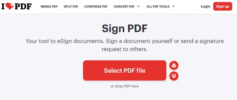
- Paso 1: Navegue hasta la herramienta Firmar PDF de iLovePDF en un navegador web y haga clic en Seleccionar archivo PDF para cargar un documento PDF.
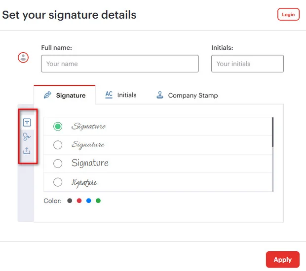
- Paso 2: Elija el tipo de firmante (por ejemplo, "Solo yo") y cree su firma dibujándola, escribiendo su nombre o cargando una imagen PNG de su firma física.
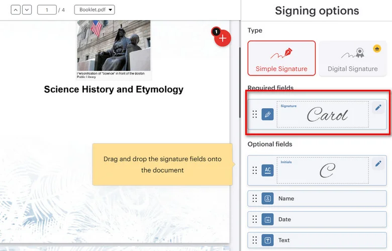
- Paso 3: Arrastre y suelte el campo de firma en la ubicación de destino en la página del PDF.
- Paso 4: Haga clic en Firmar y descargue el documento firmado.
Limitaciones: Las herramientas web solo generan firmas electrónicas visuales básicas, y cargar archivos en servidores en la nube de terceros conlleva riesgos de fuga de datos.
Cómo firmar un PDF gratis usando herramientas de escritorio integradas
Si prefiere mantener sus archivos en su ordenador, las herramientas de escritorio integradas ofrecen otra opción. Microsoft Edge en Windows le permite anotar PDF con una firma manuscrita, mientras que Vista Previa de macOS ofrece una herramienta Firmar integrada para añadir firmas electrónicas de forma local.
Microsoft Edge en Windows
Microsoft Edge incluye herramientas de anotación de PDF que le permiten dibujar una firma manuscrita directamente en un PDF. Esto añade una capa de anotación visual en lugar de una firma digital basada en certificados.
- Paso 1: Haga clic con el botón derecho en un documento PDF y seleccione Abrir con > Microsoft Edge.
- Paso 2: Haga clic en el icono Dibujar (símbolo de bolígrafo) en la barra de herramientas superior.
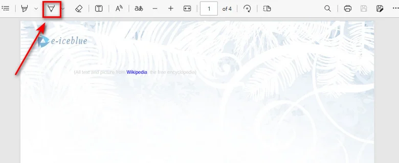
- Paso 3: Utilice el ratón, el panel táctil o el lápiz óptico para dibujar su firma directamente en el documento.
- Paso 4: Haga clic en el botón Guardar para guardar el PDF anotado.
Vista Previa de macOS
Vista Previa de macOS proporciona una herramienta de firma integrada que le permite crear y añadir una firma manuscrita a un PDF localmente.
- Paso 1: Haga doble clic en su archivo PDF para abrirlo en Vista Previa de macOS.
- Paso 2: Haga clic en el botón Barra de herramientas de marcación (icono de bolígrafo) en el menú superior y, a continuación, seleccione la herramienta Firmar.
- Paso 3: Cree una firma utilizando su trackpad, escaneando una firma en papel con la cámara de su Mac o escribiendo en un iPhone/iPad conectado.
- Paso 4: Haga clic en la firma guardada para insertarla, arrástrela a la línea correcta y guarde el PDF mediante Archivo > Guardar o Cmd + S.
Limitaciones: Estas herramientas integradas no crean firmas digitales basadas en certificados. Microsoft Edge ofrece principalmente funciones de anotación en PDF, mientras que Vista Previa de macOS añade elementos de firma electrónica. Ambos métodos requieren un procesamiento manual archivo por archivo, lo que los hace inadecuados para la firma por lotes o flujos de trabajo automatizados.
Cómo firmar digitalmente un PDF sin Adobe usando Python (Procesamiento por lotes)
Al crear backends web, sistemas de facturación automatizados o microservicios empresariales, las herramientas manuales de arrastrar y soltar resultan insuficientes. Los desarrolladores necesitan una solución que pueda firmar digitalmente archivos PDF sin Adobe manteniendo la privacidad de los datos y un control total del backend.
Free Spire.PDF para Python es una librería independiente y ligera que permite a los desarrolladores procesar y firmar documentos PDF sin depender de Adobe Acrobat. Admite certificados digitales almacenados en archivos PKCS#12 (.pfx o .p12).
Añadir una firma digital invisible a un PDF
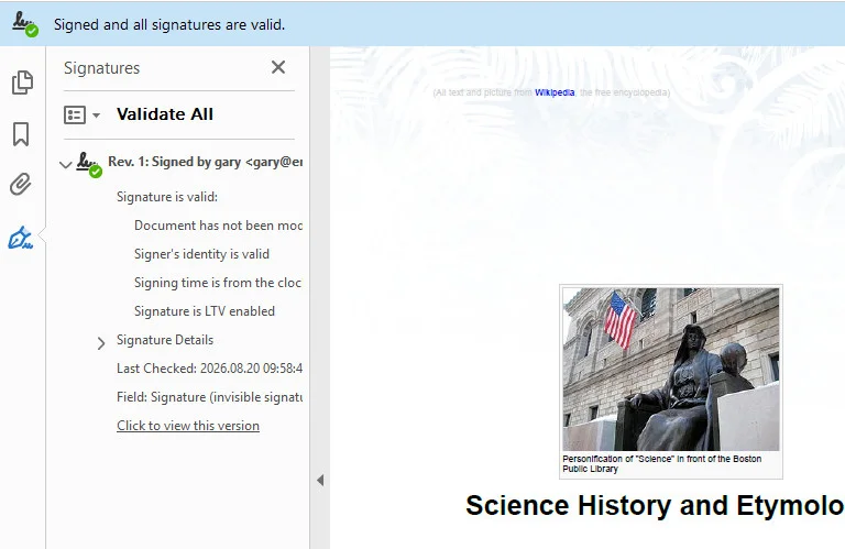
Una firma digital invisible aplica una firma criptográfica a un PDF sin mostrar una apariencia de firma en la página. Con Free Spire.PDF para Python, puede utilizar PdfOrdinarySignatureMaker para cargar un certificado PKCS#12 (.pfx o .p12) y aplicar la firma al documento.
En el siguiente ejemplo, la ruta del certificado y la contraseña se pasan a PdfOrdinarySignatureMaker, que crea la firma digital sin añadir una apariencia de firma visible.
from spire.pdf.common import *
from spire.pdf import *

# Crear una nueva instancia de PdfDocument
doc = PdfDocument()
# Cargar un documento PDF
doc.LoadFromFile("/input/Booklet.pdf")

# Crear una instancia de PdfOrdinarySignatureMaker
signatureMaker = PdfOrdinarySignatureMaker(doc, "/gary.pfx", "e-iceblue")

# Añadir una firma digital invisible al documento
signatureMaker.MakeSignature("Signature")

# Guardar el documento PDF firmado
doc.SaveToFile("/output/invisible signature.pdf")
doc.Close()
Añadir una firma digital visible a un PDF
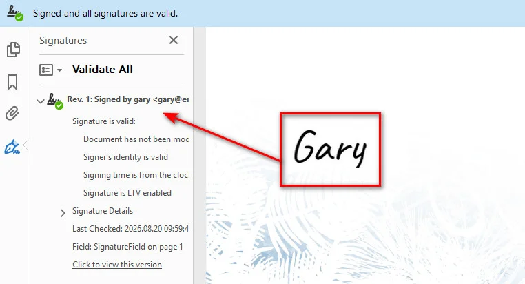
Una firma digital visible combina un sello gráfico en la página (como un sello oficial o una imagen de firma) con un sello criptográfico PKI. La apariencia visual se configura con PdfSignatureAppearance, mientras que SignatureImage especifica la imagen de la firma y MakeSignature() define la página y la posición de la firma visible.
from spire.pdf import *

# Paso 1: Cargar el documento PDF de destino
doc = PdfDocument()
doc.LoadFromFile("/input/Booklet.pdf")

# Paso 2: Inicializar el creador de firmas con la ruta del certificado y la contraseña
signatureMaker = PdfOrdinarySignatureMaker(doc, "/gary.pfx", "e-iceblue")

# Paso 3: Configurar los metadatos de la firma
signature = signatureMaker.Signature
signature.Name = "Finance Department"
signature.ContactInfo = "finance@company.com"
signature.Reason = "Approved for Payment"

# Paso 4: Configurar la apariencia visual y adjuntar la imagen del sello
appearance = PdfSignatureAppearance(signature)
appearance.SignatureImage = PdfImage.FromFile("/gary sign.png")
appearance.GraphicMode = GraphicMode.SignImageOnly

# Paso 5: Aplicar la firma en la página 1 en las coordenadas de destino (X, Y, Ancho, Alto)
page = doc.Pages[0]
signatureMaker.MakeSignature("SignatureField", page, 100.0, 600.0, 180.0, 60.0, appearance)

# Paso 6: Guardar el documento PDF firmado
doc.SaveToFile("/output/signed_visible.pdf")
doc.Close()
Nota: Después de firmar un PDF, es posible que también necesite verificar la firma o extraer la información de la firma para auditorías y validación de documentos. Consulte Python: Verificar y extraer firmas digitales en PDF para conocer un enfoque programático.
Cómo elegir su solución para firmar PDF
Elegir el método adecuado para firmar PDF depende de sus requisitos de privacidad, sus habilidades técnicas y la escala de su flujo de trabajo. Compare las características clave a continuación para encontrar el enfoque que mejor se adapte a su configuración:
| Característica | iLovePDF (Herramienta web) | Vista Previa de macOS / Edge (Nativo del SO) | Free Spire.PDF para Python (SDK) |
|---|---|---|---|
| Tipo de firma | Firma electrónica (Básica) | Firma electrónica | Firma digital basada en certificados |
| Facilidad de uso | Instantánea (Navegador) | Alta (Preinstalado) | Media (Habilidades de desarrollador) |
| Privacidad de datos | Menor (Carga en la nube) | Alta (Ejecución local) | Alta (Ejecución local/servidor) |
| Automatización | Baja (Manual) | Baja (Manual) | Alta (Flujos de trabajo automatizados) |
| Seguridad | Depende del método de firma | Firma electrónica básica | Firma criptográfica basada en certificados |
Conclusión
No necesita Adobe Acrobat para añadir una firma a un PDF. Para una firma electrónica rápida, una herramienta en línea o una aplicación de escritorio integrada suele ser suficiente. Si necesita una firma digital basada en certificados o un procesamiento automatizado, una biblioteca de PDF para Python ofrece un mayor control sobre el flujo de trabajo de firma.
El enfoque adecuado depende de cómo planee utilizar el documento firmado. Elija una herramienta local cuando la privacidad del documento sea importante, un servicio en línea cuando la comodidad sea lo más relevante, o una solución basada en Python cuando la firma deba integrarse en una aplicación automatizada.
Lea también:
Wie man ein PDF ohne Adobe signiert: 3 kostenlose Methoden
Inhaltsverzeichnis
Adobe Acrobat ist seit Langem eine beliebte Wahl für die Verwaltung von PDF-Dokumenten, aber die Abonnementkosten und die Anforderungen an Desktop-Software sind möglicherweise nicht für jeden ideal. Glücklicherweise können Sie eine PDF-Datei ohne Adobe signieren, indem Sie mehrere einfachere Alternativen nutzen.
Dieser Leitfaden führt Sie durch drei praktische Ansätze: das Signieren einer PDF-Datei mit einem Online-Tool, das lokale Hinzufügen einer Signatur mit integrierten Desktop-Apps und das Anwenden einer zertifikatsbasierten digitalen Signatur mit Python. Jede Methode enthält Schritt-für-Schritt-Anleitungen, sodass Sie die Option auswählen können, die Ihren Anforderungen am besten entspricht.
- PDF-Signaturen verstehen: Elektronisch vs. Digital
- So signieren Sie eine PDF-Datei ohne Adobe mit iLovePDF
- So signieren Sie eine PDF-Datei kostenlos mit integrierten Desktop-Tools
- So signieren Sie eine PDF-Datei digital ohne Adobe mit Python (Stapelverarbeitung)
- Wählen Sie Ihre PDF-Signaturlösung
PDF-Signaturen verstehen: Elektronisch vs. Digital
Bevor Sie sich für ein Tool entscheiden, ist es hilfreich zu verstehen, was beim Signieren einer PDF-Datei passiert.
- Elektronische Signaturen (E-Signaturen): Eine elektronische Signatur kann durch einen eingegebenen Namen, eine gezeichnete Signatur, ein hochgeladenes Bild oder andere elektronische Signaturdaten dargestellt werden, die einem Dokument hinzugefügt werden.
- Digitale Signaturen: Eine digitale PDF-Signatur verwendet ein digitales Zertifikat und kryptografische Algorithmen, um den Unterzeichner zu authentifizieren und Änderungen am Dokument nach der Unterzeichnung zu erkennen.
Digitale PDF-Signaturen können unsichtbar sein, was bedeutet, dass die kryptografische Signatur in der PDF-Datei ohne sichtbares Erscheinungsbild gespeichert wird, oder sichtbar, was bedeutet, dass die kryptografische Signatur von einem visuellen Signaturbild auf der Seite begleitet wird.
So signieren Sie eine PDF-Datei ohne Adobe mit iLovePDF
Für gelegentliche Signaturaufgaben bieten browserbasierte PDF-Editoren eine praktische Option, ohne dass zusätzliche Software erforderlich ist. Plattformen wie iLovePDF ermöglichen es Ihnen, eine PDF-Datei hochzuladen, eine Signatur durch Zeichnen, Tippen oder Hochladen eines Bildes zu erstellen und das signierte Dokument direkt aus Ihrem Browser zu exportieren. Für die kostenlose oder grundlegende Nutzung konzentrieren sich Online-Signatur-Tools in der Regel auf elektronische Signaturen, während zertifikatsbasiertes digitales Signieren möglicherweise einen kostenpflichtigen Tarif erfordert.
Hier sind die Schritte zum Signieren einer PDF-Datei mit iLovePDF:
- Schritt 1: Navigieren Sie im Webbrowser zum Werkzeug PDF signieren von iLovePDF und klicken Sie auf PDF-Datei auswählen, um ein PDF-Dokument hochzuladen.
- Schritt 2: Wählen Sie Ihren Unterzeichnertyp (z. B. „Nur ich“) und erstellen Sie Ihre Signatur, indem Sie sie zeichnen, Ihren Namen eingeben oder ein PNG-Bild Ihrer handschriftlichen Unterschrift hochladen.
- Schritt 3: Ziehen Sie Ihr Signaturfeld per Drag-and-Drop an die gewünschte Stelle auf der PDF-Seite.
- Schritt 4: Klicken Sie auf Signieren und laden Sie das signierte Dokument herunter.
Einschränkungen: Web-Tools erzeugen nur grundlegende visuelle E-Signaturen, und das Hochladen von Dateien auf Cloud-Server von Drittanbietern birgt Risiken von Datenlecks.
So signieren Sie eine PDF-Datei kostenlos mit integrierten Desktop-Tools
Wenn Sie Ihre Dateien lieber auf Ihrem Computer behalten möchten, bieten integrierte Desktop-Tools eine weitere Option. Mit Microsoft Edge unter Windows können Sie PDFs mit einer handschriftlichen Unterschrift versehen, während die Vorschau unter macOS ein integriertes Signatur-Tool zum lokalen Hinzufügen elektronischer Signaturen bereitstellt.
Windows Microsoft Edge
Microsoft Edge enthält PDF-Anmerkungstools, mit denen Sie eine handschriftliche Unterschrift direkt auf einer PDF-Datei zeichnen können. Dadurch wird eher eine visuelle Anmerkungsebene als eine zertifikatsbasierte digitale Signatur hinzugefügt.
- Schritt 1: Klicken Sie mit der rechten Maustaste auf ein PDF-Dokument und wählen Sie Öffnen mit > Microsoft Edge.
- Schritt 2: Klicken Sie in der oberen Symbolleiste auf das Symbol Zeichnen (Stiftsymbol).
- Schritt 3: Verwenden Sie Ihre Maus, Ihr Touchpad oder einen Stift, um Ihre Unterschrift direkt auf das Dokument zu zeichnen.
- Schritt 4: Klicken Sie auf die Schaltfläche Speichern, um die mit Anmerkungen versehene PDF-Datei zu speichern.
macOS Vorschau
Die macOS Vorschau bietet ein integriertes Signatur-Tool, mit dem Sie lokal eine handschriftliche Unterschrift erstellen und zu einer PDF-Datei hinzufügen können.
- Schritt 1: Doppelklicken Sie auf Ihre PDF-Datei, um sie in der macOS Vorschau zu öffnen.
- Schritt 2: Klicken Sie im oberen Menü auf die Schaltfläche Werkzeugleiste für Anmerkungen (Stiftsymbol) und wählen Sie dann das Werkzeug Signieren aus.
- Schritt 3: Erstellen Sie eine Signatur mit Ihrem Trackpad, indem Sie eine Unterschrift auf Papier mit der Kamera Ihres Macs scannen oder auf einem angeschlossenen iPhone/iPad schreiben.
- Schritt 4: Klicken Sie auf die gespeicherte Signatur, um sie einzufügen, ziehen Sie sie an die richtige Stelle und speichern Sie die PDF-Datei über Ablage > Sichern oder Cmd + S.
Einschränkungen: Diese integrierten Tools erstellen keine zertifikatsbasierten digitalen Signaturen. Microsoft Edge bietet hauptsächlich PDF-Anmerkungsfunktionen, während macOS Vorschau elektronische Signaturelemente hinzufügt. Beide Methoden erfordern eine manuelle Verarbeitung Datei für Datei, wodurch sie für Stapelsignierungen oder automatisierte Arbeitsabläufe ungeeignet sind.
So signieren Sie eine PDF-Datei digital ohne Adobe mit Python (Stapelverarbeitung)
Beim Aufbau von Web-Backends, automatisierten Rechnungsstellungssystemen oder Enterprise-Microservices stoßen manuelle Drag-and-Drop-Tools an ihre Grenzen. Entwickler benötigen eine Lösung, mit der sie PDFs ohne Adobe digital signieren können, während Datenschutz und die vollständige Kontrolle über das Backend gewahrt bleiben.
Free Spire.PDF for Python ist eine eigenständige, leichtgewichtige Bibliothek, die es Entwicklern ermöglicht, PDF-Dokumente zu verarbeiten und zu signieren, ohne auf Adobe Acrobat angewiesen zu sein. Sie unterstützt digitale Zertifikate, die in PKCS#12-Dateien (.pfx oder .p12) gespeichert sind.
Eine unsichtbare digitale Signatur zu einer PDF-Datei hinzufügen
Eine unsichtbare digitale Signatur wendet eine kryptografische Signatur auf eine PDF-Datei an, ohne ein visuelles Erscheinungsbild der Signatur auf der Seite anzuzeigen. Mit Free Spire.PDF for Python können Sie PdfOrdinarySignatureMaker verwenden, um ein PKCS#12-Zertifikat (.pfx oder .p12) zu laden und die Signatur auf das Dokument anzuwenden.
Im folgenden Beispiel werden Zertifikatspfad und Passwort an PdfOrdinarySignatureMaker übergeben, wodurch die digitale Signatur erstellt wird, ohne ein sichtbares Signaturbild hinzuzufügen.
from spire.pdf.common import *
from spire.pdf import *

# Eine neue PdfDocument-Instanz erstellen
doc = PdfDocument()
# Ein PDF-Dokument laden
doc.LoadFromFile("/input/Booklet.pdf")

# Eine PdfOrdinarySignatureMaker-Instanz erstellen
signatureMaker = PdfOrdinarySignatureMaker(doc, "/gary.pfx", "e-iceblue")

# Eine unsichtbare digitale Signatur zum Dokument hinzufügen
signatureMaker.MakeSignature("Signature")

# Das signierte PDF-Dokument speichern
doc.SaveToFile("/output/invisible signature.pdf")
doc.Close()
Eine sichtbare digitale Signatur zu einer PDF-Datei hinzufügen
Eine sichtbare digitale Signatur kombiniert einen grafischen Stempel auf der Seite (z. B. ein offizielles Siegel oder ein Unterschriftenbild) mit einem kryptografischen PKI-Siegel. Das visuelle Erscheinungsbild wird mit PdfSignatureAppearance konfiguriert, während SignatureImage das Signaturbild angibt und MakeSignature() die Seite und Position der sichtbaren Signatur festlegt.
from spire.pdf import *

# Schritt 1: Das Ziel-PDF-Dokument laden
doc = PdfDocument()
doc.LoadFromFile("/input/Booklet.pdf")

# Schritt 2: Signaturersteller mit Zertifikatspfad und Passwort initialisieren
signatureMaker = PdfOrdinarySignatureMaker(doc, "/gary.pfx", "e-iceblue")

# Schritt 3: Signatur-Metadaten konfigurieren
signature = signatureMaker.Signature
signature.Name = "Finance Department"
signature.ContactInfo = "finance@company.com"
signature.Reason = "Approved for Payment"

# Schritt 4: Visuelles Erscheinungsbild konfigurieren und Stempelbild anhängen
appearance = PdfSignatureAppearance(signature)
appearance.SignatureImage = PdfImage.FromFile("/gary sign.png")
appearance.GraphicMode = GraphicMode.SignImageOnly

# Schritt 5: Die Signatur auf Seite 1 an den Zielkoordinaten (X, Y, Breite, Höhe) anwenden
page = doc.Pages[0]
signatureMaker.MakeSignature("SignatureField", page, 100.0, 600.0, 180.0, 60.0, appearance)

# Schritt 6: Das signierte PDF-Dokument speichern
doc.SaveToFile("/output/signed_visible.pdf")
doc.Close()
Hinweis: Nach dem Signieren einer PDF-Datei müssen Sie möglicherweise auch die Signatur überprüfen oder Signaturinformationen für Audits und die Dokumentenvalidierung extrahieren. Siehe Python: Digitale Signaturen in PDF überprüfen und extrahieren für einen programmgesteuerten Ansatz.
Wählen Sie Ihre PDF-Signaturlösung
Die Wahl der richtigen PDF-Signaturmethode hängt von Ihren Datenschutzanforderungen, technischen Kenntnissen und dem Umfang Ihres Arbeitsablaufs ab. Vergleichen Sie die folgenden Hauptmerkmale, um den Ansatz zu finden, der am besten zu Ihren Anforderungen passt:
| Funktion | iLovePDF (Web-Tool) | macOS Vorschau / Edge (Betriebssystem-integriert) | Free Spire.PDF for Python (SDK) |
|---|---|---|---|
| Signaturtyp | Elektronische Signatur (Einfach) | Elektronische Signatur | Zertifikatsbasierte digitale Signatur |
| Benutzerfreundlichkeit | Sofort (Browser) | Hoch (Vorinstalliert) | Mittel (Entwicklerkenntnisse) |
| Datenschutz | Geringer (Cloud-Upload) | Hoch (Lokale Ausführung) | Hoch (Lokale/Server-Ausführung) |
| Automatisierung | Niedrig (Manuell) | Niedrig (Manuell) | Hoch (Automatisierte Arbeitsabläufe) |
| Sicherheit | Abhängig von der Signaturmethode | Einfaches elektronisches Signieren | Zertifikatsbasiertes kryptografisches Signieren |
Fazit
Sie benötigen keinen Adobe Acrobat, um einer PDF-Datei eine Signatur hinzuzufügen. Für eine schnelle elektronische Signatur reicht in der Regel ein Online-Tool oder eine integrierte Desktop-Anwendung aus. Wenn Sie eine zertifikatsbasierte digitale Signatur oder eine automatisierte Verarbeitung benötigen, bietet eine Python-PDF-Bibliothek eine größere Kontrolle über den Signatur-Arbeitsablauf.
Der richtige Ansatz hängt davon ab, wie Sie das signierte Dokument verwenden möchten. Wählen Sie ein lokales Tool, wenn der Datenschutz von Dokumenten wichtig ist, einen Online-Dienst, wenn Bequemlichkeit an erster Stelle steht, oder eine Python-basierte Lösung, wenn das Signieren in eine automatisierte Anwendung integriert werden muss.
Lesen Sie auch:
Как подписать PDF без Adobe: 3 бесплатных способа
```html
Содержание
Adobe Acrobat долгое время был популярным выбором для управления документами PDF, однако стоимость подписки и требования к настольному ПО могут подойти не всем. К счастью, вы можете подписать PDF без Adobe, используя несколько более простых альтернатив.
В этом руководстве рассмотрены три практических подхода: подписание PDF с помощью онлайн-инструмента, добавление подписи локально с помощью встроенных настольных приложений и наложение цифровой подписи на основе сертификата с помощью Python. Каждый метод содержит пошаговые инструкции, чтобы вы могли выбрать наиболее подходящий вариант.
- Понимание подписей PDF: электронная против цифровой
- Как подписать PDF без Adobe с помощью iLovePDF
- Как бесплатно подписать PDF с помощью встроенных настольных инструментов
- Как цифровой подписью подписать PDF без Adobe с помощью Python (пакетная обработка)
- Выбор решения для подписания PDF
Понимание подписей PDF: электронная против цифровой
Прежде чем выбирать инструмент, полезно понять, что происходит при подписании PDF-файла.
- Электронные подписи (e-Signatures): Электронная подпись может быть представлена введенным именем, нарисованной подписью, загруженным изображением или другими электронными данными подписи, добавленными в документ.
- Цифровые подписи: Цифровая подпись PDF использует цифровой сертификат и криптографические алгоритмы для проверки подлинности подписавшего и обнаружения изменений, внесенных в документ после подписания.
Цифровые подписи PDF могут быть невидимыми, то есть криптографическая подпись сохраняется в PDF без визуального отображения, или видимыми, то есть криптографическая подпись сопровождается визуальным отображением подписи на странице.
Как подписать PDF без Adobe с помощью iLovePDF
Для периодических задач по подписанию онлайн-редакторы PDF предлагают удобный вариант, не требующий установки дополнительного ПО. Платформы, такие как iLovePDF, позволяют загружать PDF, создавать подпись путем рисования, ввода текста или загрузки изображения, а также экспортировать подписанный документ прямо из браузера. Для бесплатного или базового использования онлайн-инструменты обычно ориентированы на электронные подписи, тогда как цифровая подпись на основе сертификата может потребовать платного тарифа.
Вот шаги для подписания PDF с помощью iLovePDF:
- Шаг 1: Перейдите к инструменту iLovePDF Sign PDF в веб-браузере и нажмите Select PDF file, чтобы загрузить PDF-документ.
- Шаг 2: Выберите тип подписанта (например, "Only me") и создайте подпись, нарисовав ее, введя свое имя или загрузив PNG-изображение вашей обычной подписи.
- Шаг 3: Перетащите поле подписи в нужное место на странице PDF.
- Шаг 4: Нажмите Sign и скачайте подписанный документ.
Ограничения: Веб-инструменты создают только базовые визуальные электронные подписи, а загрузка файлов на сторонние облачные серверы сопряжена с рисками утечки данных.
Как бесплатно подписать PDF с помощью встроенных настольных инструментов
Если вы предпочитаете хранить файлы на своем компьютере, отличной альтернативой станут встроенные настольные инструменты. Microsoft Edge в Windows позволяет аннотировать PDF-файлы рукописной подписью, а программа «Просмотр» (Preview) в macOS предоставляет встроенный инструмент подписи для локального добавления электронных подписей.
Windows Microsoft Edge
Microsoft Edge содержит инструменты разметки PDF, которые позволяют рисовать рукописную подпись непосредственно на PDF-документе. Это добавляет слой визуальных аннотаций, а не цифровую подпись на основе сертификата.
- Шаг 1: Нажмите правой кнопкой мыши на PDF-документ и выберите Открыть с помощью > Microsoft Edge.
- Шаг 2: Нажмите иконку Рисовать (символ пера) на верхней панели инструментов.
- Шаг 3: Используйте мышь, трекпад или стилус, чтобы нарисовать подпись прямо на документе.
- Шаг 4: Нажмите кнопку Сохранить, чтобы сохранить PDF с аннотацией.
macOS Preview
Приложение «Просмотр» (Preview) в macOS содержит встроенный инструмент подписи, позволяющий локально создавать и добавлять рукописную подпись в PDF.
- Шаг 1: Двойным кликом откройте PDF-файл в приложении macOS Preview.
- Шаг 2: Нажмите кнопку Панель инструментов разметки (иконка пера) в верхнем меню, затем выберите инструмент Подписать.
- Шаг 3: Создайте подпись с помощью трекпада, отсканировав бумажную подпись камерой Mac или написав ее на подключенном iPhone/iPad.
- Шаг 4: Нажмите на сохраненную подпись, чтобы вставить ее, перетащите на нужную строку и сохраните PDF с помощью Файл > Сохранить или комбинации клавиш Cmd + S.
Ограничения: Эти встроенные инструменты не создают цифровых подписей на основе сертификатов. Microsoft Edge в основном предоставляет функции разметки PDF, а приложение «Просмотр» в macOS добавляет элементы электронной подписи. Оба метода требуют ручной обработки по одному файлу за раз, что делает их непригодными для пакетного подписания или автоматизированных рабочих процессов.
Как цифровой подписью подписать PDF без Adobe с помощью Python (пакетная обработка)
При создании веб-бэкендов, автоматизированных систем выставления счетов или корпоративных микросервисов ручные инструменты с перетаскиванием оказываются недостаточными. Разработчикам требуется решение, способное подписывать PDF-файлы цифровой подписью без Adobe, сохраняя при этом конфиденциальность данных и полный контроль над бэкендом.
Free Spire.PDF for Python — это автономная облегченная библиотека, которая позволяет разработчикам обрабатывать и подписывать PDF-документы без использования Adobe Acrobat. Она поддерживает цифровые сертификаты, хранящиеся в файлах PKCS#12 (.pfx или .p12).
Добавление невидимой цифровой подписи в PDF
Невидимая цифровая подпись применяет криптографическую подпись к PDF без отображения внешнего вида подписи на странице. С помощью Free Spire.PDF для Python вы можете использовать PdfOrdinarySignatureMaker для загрузки сертификата PKCS#12 (.pfx или .p12) и применения подписи к документу.
В следующем примере путь к сертификату и пароль передаются в PdfOrdinarySignatureMaker, который создает цифровую подпись без добавления видимого отображения.
from spire.pdf.common import *
from spire.pdf import *

# Create a new PdfDocument instance
doc = PdfDocument()
# Load a PDF document
doc.LoadFromFile("/input/Booklet.pdf")

# Create a PdfOrdinarySignatureMaker instance
signatureMaker = PdfOrdinarySignatureMaker(doc, "/gary.pfx", "e-iceblue")

# Add an invisible digital signature to the document
signatureMaker.MakeSignature("Signature")

# Save the signed PDF document
doc.SaveToFile("/output/invisible signature.pdf")
doc.Close()
Добавление видимой цифровой подписи в PDF
Видимая цифровая подпись сочетает в себе графический штамп на странице (например, официальную печать или изображение подписи) с криптографической печатью PKI. Визуальный вид настраивается с помощью PdfSignatureAppearance, параметр SignatureImage задает изображение подписи, а метод MakeSignature() определяет страницу и позицию видимой подписи.
from spire.pdf import *

# Step 1: Load the target PDF document
doc = PdfDocument()
doc.LoadFromFile("/input/Booklet.pdf")

# Step 2: Initialize signature maker with certificate path and password
signatureMaker = PdfOrdinarySignatureMaker(doc, "/gary.pfx", "e-iceblue")

# Step 3: Configure signature metadata
signature = signatureMaker.Signature
signature.Name = "Finance Department"
signature.ContactInfo = "finance@company.com"
signature.Reason = "Approved for Payment"

# Step 4: Configure visual appearance and attach stamp image
appearance = PdfSignatureAppearance(signature)
appearance.SignatureImage = PdfImage.FromFile("/gary sign.png")
appearance.GraphicMode = GraphicMode.SignImageOnly

# Step 5: Apply the signature to page 1 at target coordinates (X, Y, Width, Height)
page = doc.Pages[0]
signatureMaker.MakeSignature("SignatureField", page, 100.0, 600.0, 180.0, 60.0, appearance)

# Step 6: Save the signed PDF document
doc.SaveToFile("/output/signed_visible.pdf")
doc.Close()
Примечание. После подписания PDF вам также может потребоваться проверить подпись или извлечь информацию о ней для аудита и проверки документа. Ознакомьтесь со статьей Python: проверка и извлечение цифровых подписей в PDF для программного подхода.
Выбор решения для подписания PDF
Выбор правильного метода подписания PDF зависит от ваших требований к конфиденциальности, технических навыков и масштаба рабочего процесса. Сравните ключевые функции ниже, чтобы найти подход, наиболее подходящий для ваших задач:
| Функция | iLovePDF (Веб-инструмент) | macOS Preview / Edge (Встроенные в ОС) | Free Spire.PDF for Python (SDK) |
|---|---|---|---|
| Тип подписи | Электронная подпись (базовая) | Электронная подпись | Цифровая подпись на основе сертификата |
| Удобство использования | Мгновенно (браузер) | Высокое (предустановлено) | Среднее (навыки разработчика) |
| Конфиденциальность данных | Ниже (загрузка в облако) | Высокая (локальное выполнение) | Высокая (локальное/серверное выполнение) |
| Автоматизация | Низкая (вручную) | Низкая (вручную) | Высокая (автоматизированные процессы) |
| Безопасность | Зависит от метода подписания | Базовое электронное подписание | Криптографическая подпись на основе сертификата |
Заключение
Вам не нужен Adobe Acrobat, чтобы добавить подпись в PDF. Для быстрого создания электронной подписи обычно достаточно онлайн-инструмента или встроенного настольного приложения. Если вам нужна цифровая подпись на основе сертификата или автоматизированная обработка, библиотека Python для PDF обеспечит больший контроль над процессом подписания.
Правильный подход зависит от того, как вы планируете использовать подписанный документ. Выбирайте локальный инструмент, если важна конфиденциальность документа, онлайн-сервис, если превыше всего удобство, или решение на базе Python, если подписание необходимо интегрировать в автоматизированное приложение.
Читайте также:
```
Inserir segmentações de dados no Excel: Guia para iniciantes sobre filtros interativos
Sumário
- O que é um Segmentador de Dados (Slicer) no Excel?
- Por que os Segmentadores superam os filtros tradicionais
- Pré-requisitos antes de inserir Segmentadores
- Como adicionar Segmentadores no Excel: Dois métodos
- Avançado: Criar Segmentadores programaticamente no Excel com C#
- Como usar os Segmentadores do Excel após inseri-los
- Melhores práticas para Segmentadores do Excel
- Perguntas Frequentes (FAQs)
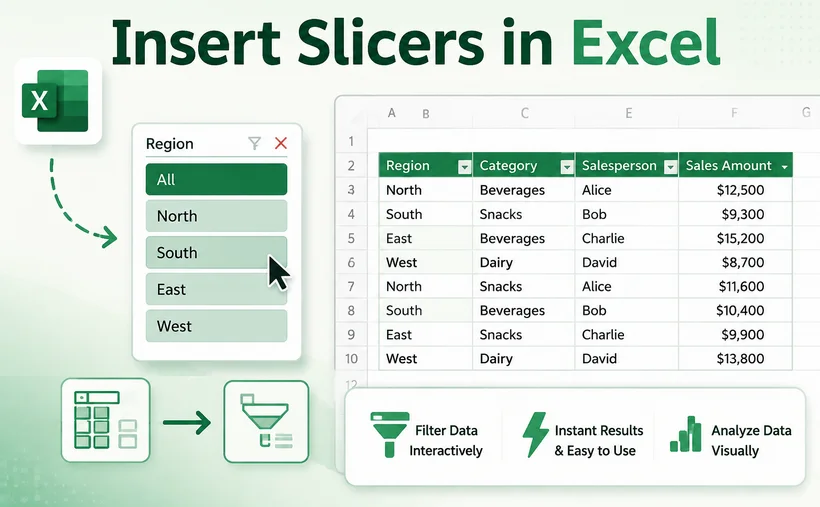
Cansado de perder o controle dos seus filtros do Excel dentro de menus suspensos intermináveis? Existe uma maneira melhor. Os Segmentadores de Dados (Slicers) transformam a exploração de dados tediosa em uma experiência visual de um clique, mantendo suas seleções visíveis e seus painéis interativos.
Neste guia, você aprenderá exatamente como inserir segmentadores no Excel, esteja você trabalhando com tabelas ou Tabelas Dinâmicas. Abordaremos as melhores práticas para criar painéis profissionais e até mostraremos como automatizar o processo com C#.
- O que é um Segmentador de Dados no Excel?
- Por que os Segmentadores superam os filtros tradicionais
- Pré-requisitos antes de inserir Segmentadores
- Como adicionar Segmentadores no Excel: Dois métodos
- Avançado: Criar Segmentadores programaticamente no Excel com C#
- Como usar os Segmentadores do Excel após inseri-los
- Melhores práticas para Segmentadores do Excel
- Perguntas Frequentes (FAQs)
O que é um Segmentador de Dados no Excel?
Um segmentador é uma ferramenta de filtragem visual composta por botões clicáveis que correspondem a valores únicos em uma coluna de dados. Em vez de ocultar suas opções de filtro dentro de menus suspensos, os segmentadores as exibem diretamente na sua planilha, tornando o estado atual do filtro visível rapidamente.
Pense nos segmentadores como um painel de controle intuitivo para seus dados. Clique em um botão e sua tabela, Tabela Dinâmica ou gráfico será atualizado instantaneamente. Os botões selecionados permanecem destacados, para que você e qualquer outro usuário possam sempre ver quais filtros estão ativos.
Por que os Segmentadores superam os filtros tradicionais
| Recurso | Filtros Tradicionais | Segmentadores |
|---|---|---|
| Visibilidade | O estado do filtro fica oculto em menus suspensos | Os filtros selecionados estão sempre visíveis |
| Facilidade de uso | Requer vários cliques para navegar pelas camadas do menu | Seleção de botão com um clique para filtragem instantânea |
| Seleção múltipla | Desajeitada e pouco intuitiva | Segure Ctrl ou use a alternância de Seleção Múltipla |
| Múltiplas fontes de dados | Vinculado a uma única tabela | Pode controlar múltiplas Tabelas Dinâmicas e gráficos |
| Amigável para painéis | Não projetado para painéis | Perfeito para painéis interativos |
Os filtros padrão forçam você a clicar em uma pequena seta, desmarcar "Selecionar Tudo", rolar por uma longa lista e clicar em OK. No momento em que você clica fora, suas escolhas de filtro desaparecem da vista, deixando você adivinhando o que está aplicado no momento. A ferramenta de segmentação do Excel resolve esse problema completamente, tornando cada opção de filtro um botão claro e clicável que fica diretamente na sua planilha.
Pré-requisitos antes de inserir Segmentadores
Antes de adicionar segmentadores no Excel, certifique-se de que seus dados atendam a estes requisitos:
- Formatado como Tabela ou Tabela Dinâmica do Excel: Os segmentadores não funcionam com intervalos de células brutos não formatados.
- Versão do Excel compatível: Os segmentadores estão disponíveis no Excel 2013 e posterior para Windows, e Excel 2016 e posterior para Mac.
- Sem linhas ou colunas em branco: Linhas ou colunas vazias dentro do seu conjunto de dados podem fazer com que o Excel interprete mal o intervalo completo de dados.
- Dados limpos e estruturados: Certifique-se de que cada coluna tenha um cabeçalho único e descritivo e uma formatação de dados consistente.
Para converter um intervalo em uma tabela, selecione seus dados e pressione "Ctrl + T", depois clique em OK.
Como adicionar Segmentadores no Excel: Dois métodos
O processo para inserir segmentadores depende se você está trabalhando com uma Tabela do Excel comum ou uma Tabela Dinâmica. Abordaremos ambos.
Método 1: Inserir Segmentadores em uma Tabela do Excel
- Clique em qualquer lugar dentro da sua tabela do Excel.
- Vá para a guia Design da Tabela na faixa de opções.
- Clique no botão Inserir Segmentação de Dados no grupo Ferramentas.

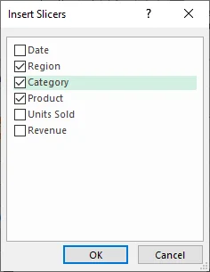
- Na caixa de diálogo pop-up, marque as caixas das colunas que você deseja usar como segmentadores (por exemplo, Região, Produto, Categoria).
- Clique em OK.
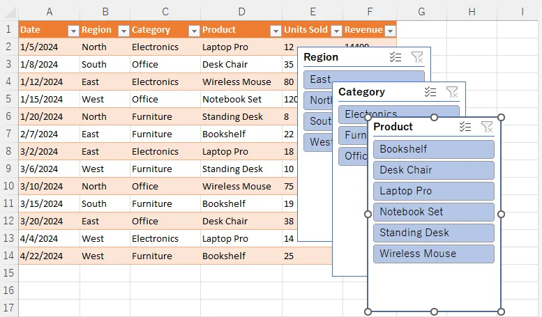
O Excel colocará objetos de segmentação diretamente na sua planilha. Cada segmentador exibe botões para todos os itens únicos em seu respectivo campo. Clique em qualquer botão dentro de um segmentador para filtrar a tabela instantaneamente.
Método 2: Inserir Segmentadores em uma Tabela Dinâmica
- Clique em qualquer célula dentro da sua tabela dinâmica.
- Navegue até a guia Análise de Tabela Dinâmica (ou guia Analisar, dependendo da sua versão).
- Clique em Inserir Segmentação de Dados no grupo Filtrar.

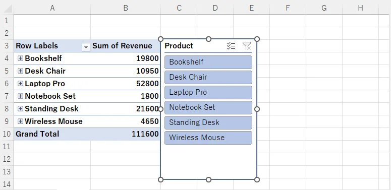
- Na caixa de diálogo Inserir Segmentação de Dados, marque as caixas dos campos pelos quais você deseja filtrar (por exemplo, Produto).
- Clique em OK.
Os segmentadores aparecem na sua planilha e atualizam dinamicamente os resultados da Tabela Dinâmica. Você pode movê-los, redimensioná-los e formatá-los para combinar com o layout do seu painel.
Avançado: Criar Segmentadores programaticamente no Excel com C#
Embora os métodos manuais sejam perfeitos para tarefas pontuais, você pode precisar adicionar segmentadores a centenas de arquivos do Excel programaticamente. É aí que entra o Free Spire.XLS for .NET. Esta biblioteca gratuita permite criar, ler e modificar arquivos do Excel sem o Microsoft Office instalado — e ela oferece suporte total à inserção de segmentadores em tabelas do Excel.
Código C#: Adicionando Segmentadores a uma Tabela do Excel
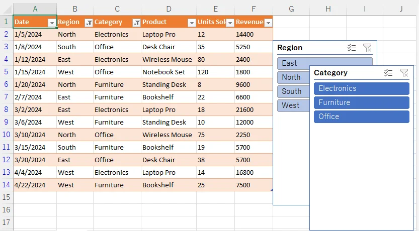
Abaixo está um exemplo completo em C# que carrega um arquivo do Excel existente, recupera a primeira tabela na primeira planilha e insere dois segmentadores para duas colunas diferentes. Em seguida, ele define um nome e um estilo integrado para cada segmentador e salva o resultado como um novo arquivo .xlsx.
using Spire.Xls;
using Spire.Xls.Core;

namespace AddSlicerToTable
{
    internal class Program
    {
        static void Main(string[] args)
        {
            // Carregar um arquivo do Excel
            Workbook workbook = new Workbook();
            workbook.LoadFromFile("sampleData.xlsx");

            // Obter a primeira planilha
            Worksheet worksheet = workbook.Worksheets[0];

            // Obter a primeira tabela na planilha
            IListObject table = worksheet.ListObjects[0];

            // Adicionar 2 segmentadores
            // Parâmetros: tabela, localização (referência de célula), índice da coluna (baseado em 0)
            int slicer1 = worksheet.Slicers.Add(table, "G3", 1);
            int slicer2 = worksheet.Slicers.Add(table, "H5", 2);

            // Definir nome e estilo para o segmentador
            worksheet.Slicers[slicer1].Name = "Região";
            worksheet.Slicers[slicer1].StyleType = SlicerStyleType.SlicerStyleLight1;
            worksheet.Slicers[slicer2].Name = "Categoria";
            worksheet.Slicers[slicer2].StyleType = SlicerStyleType.SlicerStyleDark1;

            // Salvar o arquivo de resultado
            workbook.SaveToFile("AddSlicers.xlsx", ExcelVersion.Version2016);
            workbook.Dispose();
        }
    }
}
Como funciona a API de Segmentação
O método principal é Slicers.Add() com a seguinte assinatura:
int Add(IListObject table, string destCellName, int index);
- table: O IListObject (Tabela do Excel) de origem ao qual o segmentador está vinculado
- destCellName: Endereço da célula superior esquerda onde o segmentador é colocado (por exemplo, "G3")
- index: Índice baseado em 0 da coluna dentro da tabela a ser usada como valores de filtro.
Nota: Os segmentadores exigem um objeto de Tabela do Excel estruturado. Sempre crie e configure sua tabela do Excel antes de chamar a API de inserção de segmentação.
Resultado:
Dicas adicionais para inserção programática de segmentadores
- Múltiplas tabelas: Se sua planilha tiver mais de uma tabela, você pode acessá-las via worksheet.ListObjects[index].
- Segmentadores de Tabela Dinâmica: O Free Spire.XLS também oferece suporte à adição de segmentadores a Tabelas Dinâmicas usando
worksheet.Slicers.Add(IPivotTable, string, int). - Formatos de salvamento: Use
ExcelVersion.Version2013ouVersion2016para garantir que os segmentadores sejam preservados corretamente. - Desempenho: Ao processar vários arquivos, crie uma nova instância de Workbook para cada arquivo e chame Dispose() imediatamente após o processamento para evitar vazamentos de memória.
Como usar os Segmentadores do Excel após inseri-los
Usar segmentadores é notavelmente simples:
- Seleção única: Clique em qualquer botão para filtrar seus dados para esse valor
- Seleção múltipla: Segure Ctrl enquanto clica em vários botões, ou clique na alternância Seleção Múltipla na parte superior do painel do segmentador
- Limpar um filtro: Clique no botão Limpar Filtro (o ícone de funil com um X) no canto superior direito do segmentador
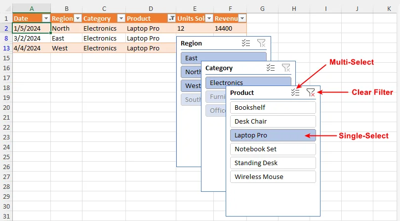
Melhores práticas para Segmentadores do Excel
- Mantenha os segmentadores agrupados e alinhados na parte superior ou lateral do seu painel.
- Use legendas descritivas para que os espectadores entendam o que cada segmentador filtra.
- Limite o número de segmentadores — 3 a 5 geralmente oferecem interatividade suficiente sem sobrecarregar.
- Nomeie seus segmentadores no Painel de Seleção (Alt + F10) para facilitar o gerenciamento.
- Bloqueie as posições dos segmentadores (clique com o botão direito → Tamanho e Propriedades → Propriedades → marque "Não mover ou dimensionar com células") para que eles permaneçam no lugar quando os usuários rolarem a página.
- Para automação, sempre direcione para ExcelVersion.Version2016 ou superior para garantir a compatibilidade do segmentador.
Considerações Finais
Adicionar segmentadores no Excel é uma das habilidades de maior impacto para quem cria relatórios ou painéis. Para usuários comuns, eles tornam a filtragem intuitiva, transparente e pronta para painéis, eliminando o atrito de menus suspensos aninhados. Para desenvolvedores, as APIs de segmentação programática permitem a geração escalável e automatizada de pastas de trabalho interativas em escala empresarial.
Não se contente com planilhas estáticas que confundem seu público. Comece a usar os segmentadores do Excel hoje para desbloquear todo o potencial dos seus dados — transformando tabelas comuns em ferramentas de tomada de decisão poderosas e interativas que impressionam e informam.
Perguntas Frequentes (FAQs)
P: Posso conectar um segmentador a várias Tabelas Dinâmicas?
R: Sim. Clique com o botão direito no segmentador → Conexões de Relatório → selecione todas as Tabelas Dinâmicas que você deseja controlar.
P: Posso alterar as cores do segmentador?
R: Com certeza. Use a guia Ferramentas de Segmentação → Opções para aplicar estilos integrados ou criar formatação personalizada.
P: Os segmentadores funcionam com gráficos do Excel?
R: Sim. Se um gráfico estiver vinculado a uma Tabela ou Tabela Dinâmica que tenha um segmentador associado, o gráfico será atualizado automaticamente para refletir suas seleções de segmentação.
P: Posso alterar a ordem de classificação dos itens dentro de um segmentador?
R: Sim. Clique com o botão direito no segmentador e selecione Configurações de Segmentação de Dados. Na caixa de diálogo, você pode escolher a ordem de classificação crescente (A-Z) ou decrescente (Z-A), ou optar por classificar usando uma lista personalizada. Você também pode controlar se os itens excluídos dos dados de origem são mantidos na exibição do segmentador.
Veja Também
Excel에서 슬라이서 삽입하기: 대화형 필터 초보자 가이드
끝없는 드롭다운 메뉴 속에서 Excel 필터를 관리하느라 지치셨나요? 더 나은 방법이 있습니다. 슬라이서(Slicers)는 번거로운 데이터 탐색 과정을 클릭 한 번으로 가능한 시각적 경험으로 바꿔주며, 선택 항목을 항상 표시하고 대시보드를 대화형으로 유지해 줍니다.
이 가이드에서는 테이블이나 피벗 테이블을 사용할 때 Excel에 슬라이서를 삽입하는 방법을 정확히 배울 수 있습니다. 전문적인 대시보드를 구축하기 위한 모범 사례를 다루고, C#을 사용하여 이 과정을 자동화하는 방법까지 보여드립니다.
- Excel의 슬라이서란 무엇인가요?
- 슬라이서가 기존 필터보다 뛰어난 이유
- 슬라이서 삽입 전 필수 조건
- Excel에서 슬라이서를 추가하는 방법: 두 가지 방법
- 고급: C#을 사용하여 Excel에서 프로그래밍 방식으로 슬라이서 만들기
- 삽입된 Excel 슬라이서 사용 방법
- Excel 슬라이서 사용을 위한 모범 사례
- 자주 묻는 질문 (FAQs)
Excel의 슬라이서란 무엇인가요?
슬라이서는 데이터 열의 고유 값에 해당하는 클릭 가능한 버튼으로 구성된 시각적 필터링 도구입니다. 필터 옵션을 드롭다운 메뉴 속에 숨기는 대신, 슬라이서는 워크시트에 직접 표시하므로 현재 필터 상태를 한눈에 확인할 수 있습니다.
슬라이서를 데이터를 위한 직관적인 제어판이라고 생각하세요. 버튼을 클릭하면 테이블, 피벗 테이블 또는 차트가 즉시 업데이트됩니다. 선택된 버튼은 강조 표시된 상태로 유지되므로, 사용자는 어떤 필터가 활성화되어 있는지 항상 알 수 있습니다.
슬라이서가 기존 필터보다 뛰어난 이유
| 기능 | 기존 필터 | 슬라이서 |
|---|---|---|
| 가시성 | 필터 상태가 드롭다운 메뉴 안에 숨겨짐 | 선택된 필터가 항상 표시됨 |
| 사용 편의성 | 메뉴 계층을 탐색하기 위해 여러 번 클릭 필요 | 클릭 한 번으로 즉시 필터링 |
| 다중 선택 | 번거롭고 직관적이지 않음 | Ctrl 키를 누르거나 다중 선택 토글 사용 |
| 다중 데이터 소스 | 하나의 테이블에만 연결됨 | 여러 피벗 테이블과 차트를 제어 가능 |
| 대시보드 친화성 | 대시보드용으로 설계되지 않음 | 대화형 대시보드에 최적 |
표준 필터는 작은 화살표를 클릭하고, "모두 선택"을 해제하고, 긴 목록을 스크롤한 뒤 확인을 눌러야 합니다. 클릭을 멈추는 순간 필터링 선택 사항이 시야에서 사라져 현재 무엇이 적용되었는지 추측해야 합니다. Excel 슬라이서 도구는 모든 필터 옵션을 워크시트에 직접 배치된 명확하고 클릭 가능한 버튼으로 만들어 이 문제를 완전히 해결합니다.
슬라이서 삽입 전 필수 조건
Excel에 슬라이서를 추가하기 전에 데이터가 다음 요구 사항을 충족하는지 확인하세요:
- Excel 테이블 또는 피벗 테이블로 서식 지정: 슬라이서는 서식이 지정되지 않은 원시 셀 범위에서는 작동하지 않습니다.
- 지원되는 Excel 버전: 슬라이서는 Windows용 Excel 2013 이상, Mac용 Excel 2016 이상에서 사용할 수 있습니다.
- 빈 행이나 열 없음: 데이터 세트 내에 빈 행이나 열이 있으면 Excel이 전체 데이터 범위를 잘못 해석할 수 있습니다.
- 깔끔하고 구조화된 데이터: 모든 열에 고유하고 설명적인 헤더가 있고 데이터 서식이 일관적인지 확인하세요.
범위를 테이블로 변환하려면 데이터를 선택하고 "Ctrl + T"를 누른 다음 확인을 클릭하세요.
Excel에서 슬라이서를 추가하는 방법: 두 가지 방법
슬라이서 삽입 과정은 일반 Excel 테이블을 사용하는지, 피벗 테이블을 사용하는지에 따라 다릅니다. 두 가지 모두 다룹니다.
방법 1: Excel 테이블에 슬라이서 삽입
- Excel 테이블 내부의 아무 곳이나 클릭합니다.
- 리본 메뉴에서 테이블 디자인 탭으로 이동합니다.
- 도구 그룹에서 슬라이서 삽입 버튼을 클릭합니다.
- 팝업 대화 상자에서 슬라이서로 사용할 열(예: 지역, 제품, 카테고리)의 확인란을 선택합니다.
- 확인을 클릭합니다.
Excel이 워크시트에 직접 슬라이서 개체를 배치합니다. 각 슬라이서는 해당 필드의 모든 고유 항목에 대한 버튼을 표시합니다. 슬라이서 내의 버튼을 클릭하면 테이블이 즉시 필터링됩니다.
방법 2: 피벗 테이블에 슬라이서 삽입
- 피벗 테이블 내부의 아무 셀이나 클릭합니다.
- 피벗 테이블 분석 탭(버전에 따라 분석 탭)으로 이동합니다.
- 필터 그룹에서 슬라이서 삽입을 클릭합니다.
- 슬라이서 삽입 대화 상자에서 필터링할 필드(예: 제품)의 확인란을 선택합니다.
- 확인을 클릭합니다.
슬라이서가 시트에 나타나며 피벗 테이블 결과를 동적으로 업데이트합니다. 대시보드 레이아웃에 맞게 이동, 크기 조정 및 서식을 지정할 수 있습니다.
고급: C#을 사용하여 Excel에서 프로그래밍 방식으로 슬라이서 만들기
수동 방법은 일회성 작업에는 완벽하지만, 수백 개의 Excel 파일에 프로그래밍 방식으로 슬라이서를 추가해야 할 수도 있습니다. 이때 Free Spire.XLS for .NET이 유용합니다. 이 무료 라이브러리를 사용하면 Microsoft Office를 설치하지 않고도 Excel 파일을 생성, 읽기 및 수정할 수 있으며, Excel 테이블에 슬라이서를 삽입하는 기능을 완벽하게 지원합니다.
C# 코드: Excel 테이블에 슬라이서 추가하기
아래는 기존 Excel 파일을 로드하고, 첫 번째 워크시트의 첫 번째 테이블을 가져와 두 개의 서로 다른 열에 대해 두 개의 슬라이서를 삽입하는 전체 C# 예제입니다. 그런 다음 각 슬라이서에 이름과 기본 제공 스타일을 설정하고 결과를 새 .xlsx 파일로 저장합니다.
using Spire.Xls;
using Spire.Xls.Core;

namespace AddSlicerToTable
{
    internal class Program
    {
        static void Main(string[] args)
        {
            // Excel 파일 로드
            Workbook workbook = new Workbook();
            workbook.LoadFromFile("sampleData.xlsx");

            // 첫 번째 워크시트 가져오기
            Worksheet worksheet = workbook.Worksheets[0];

            // 워크시트의 첫 번째 테이블 가져오기
            IListObject table = worksheet.ListObjects[0];

            // 슬라이서 2개 추가
            // 매개변수: 테이블, 위치(셀 참조), 열 인덱스(0부터 시작)
            int slicer1 = worksheet.Slicers.Add(table, "G3", 1);
            int slicer2 = worksheet.Slicers.Add(table, "H5", 2);

            // 슬라이서 이름 및 스타일 설정
            worksheet.Slicers[slicer1].Name = "Region";
            worksheet.Slicers[slicer1].StyleType = SlicerStyleType.SlicerStyleLight1;
            worksheet.Slicers[slicer2].Name = "Category";
            worksheet.Slicers[slicer2].StyleType = SlicerStyleType.SlicerStyleDark1;

            // 결과 파일 저장
            workbook.SaveToFile("AddSlicers.xlsx", ExcelVersion.Version2016);
            workbook.Dispose();
        }
    }
}
슬라이서 API 작동 방식
핵심 메서드는 다음 서명을 가진 Slicers.Add()입니다:
int Add(IListObject table, string destCellName, int index);
- table: 슬라이서가 바인딩된 소스 IListObject(Excel 테이블)
- destCellName: 슬라이서가 배치될 왼쪽 상단 셀 주소(예: "G3")
- index: 필터 값으로 사용할 테이블 내 열의 0부터 시작하는 인덱스.
참고: 슬라이서는 구조화된 Excel 테이블 개체가 필요합니다. 슬라이서 삽입 API를 호출하기 전에 항상 Excel 테이블을 생성하고 구성하세요.
결과:
프로그래밍 방식 슬라이서 삽입을 위한 추가 팁
- 다중 테이블: 워크시트에 테이블이 여러 개 있는 경우
worksheet.ListObjects[index]를 통해 액세스할 수 있습니다. - 피벗 테이블 슬라이서: Free Spire.XLS는
worksheet.Slicers.Add(IPivotTable, string, int)를 사용하여 피벗 테이블에 슬라이서를 추가하는 기능도 지원합니다. - 저장 형식: 슬라이서가 올바르게 유지되도록
ExcelVersion.Version2013또는Version2016을 사용하세요. - 성능: 여러 파일을 처리할 때는 각 파일에 대해 새 Workbook 인스턴스를 생성하고 처리 후 즉시 Dispose()를 호출하여 메모리 누수를 방지하세요.
삽입된 Excel 슬라이서 사용 방법
슬라이서 사용은 매우 간단합니다:
- 단일 선택: 버튼을 클릭하여 해당 값으로 데이터를 필터링합니다.
- 다중 선택: Ctrl 키를 누른 상태에서 여러 버튼을 클릭하거나, 슬라이서 패널 상단의 다중 선택 토글을 클릭합니다.
- 필터 지우기: 슬라이서 오른쪽 상단 모서리에 있는 필터 지우기 버튼(X 표시가 있는 깔때기 아이콘)을 클릭합니다.
Excel 슬라이서 사용을 위한 모범 사례
- 슬라이서를 대시보드 상단이나 측면에 그룹화하고 정렬해 두세요.
- 뷰어가 각 슬라이서가 무엇을 필터링하는지 이해할 수 있도록 설명적인 캡션을 사용하세요.
- 슬라이서 개수를 제한하세요. 보통 3~5개가 복잡하지 않으면서 충분한 대화형 기능을 제공합니다.
- 더 쉽게 관리할 수 있도록 선택 창(Alt + F10)에서 슬라이서 이름을 지정하세요.
- 사용자가 스크롤할 때 슬라이서가 제자리에 있도록 위치를 잠그세요(마우스 오른쪽 버튼 클릭 → 크기 및 속성 → 속성 → "셀과 함께 이동하거나 크기가 변하지 않음" 체크).
- 자동화의 경우, 슬라이서 호환성을 보장하기 위해 항상 ExcelVersion.Version2016 이상을 대상으로 하세요.
최종 생각
Excel에 슬라이서를 추가하는 것은 보고서나 대시보드를 구축하는 모든 사람에게 가장 영향력 있는 기술 중 하나입니다. 일반 사용자에게는 필터링을 직관적이고 투명하며 대시보드에 적합하게 만들어 중첩된 드롭다운 메뉴의 번거로움을 없애줍니다. 개발자에게는 프로그래밍 방식의 슬라이서 API를 통해 엔터프라이즈 규모에서 대화형 통합 문서를 확장 가능하고 자동화된 방식으로 생성할 수 있게 합니다.
청중을 혼란스럽게 하는 정적인 스프레드시트에 안주하지 마세요. 오늘부터 Excel 슬라이서를 사용하여 데이터의 잠재력을 최대한 활용하고, 평범한 테이블을 정보를 제공하고 깊은 인상을 남기는 강력한 대화형 의사결정 도구로 바꿔보세요.
자주 묻는 질문 (FAQs)
Q: 하나의 슬라이서를 여러 피벗 테이블에 연결할 수 있나요?
A: 네. 슬라이서를 마우스 오른쪽 버튼으로 클릭 → 보고서 연결 → 제어하려는 모든 피벗 테이블을 선택하세요.
Q: 슬라이서 색상을 변경할 수 있나요?
A: 물론입니다. 슬라이서 도구 → 옵션 탭을 사용하여 기본 제공 스타일을 적용하거나 사용자 지정 서식을 만드세요.
Q: 슬라이서가 Excel 차트와 작동하나요?
A: 네. 차트가 연결된 슬라이서가 있는 테이블이나 피벗 테이블에 연결되어 있으면, 차트가 슬라이서 선택 사항을 반영하여 자동으로 업데이트됩니다.
Q: 슬라이서 내 항목의 정렬 순서를 변경할 수 있나요?
A: 네. 슬라이서를 마우스 오른쪽 버튼으로 클릭하고 슬라이서 설정을 선택하세요. 대화 상자에서 오름차순(A-Z) 또는 내림차순(Z-A) 정렬 순서를 선택하거나 사용자 지정 목록을 사용하여 정렬할 수 있습니다. 또한 소스 데이터에서 삭제된 항목을 슬라이서 표시에 유지할지 여부도 제어할 수 있습니다.
참고 항목
Inserire gli slicer in Excel: Guida per principianti ai filtri interattivi
Sommario
- Cos'è uno Slicer in Excel?
- Perché gli Slicer sono superiori ai filtri tradizionali
- Prerequisiti prima di inserire gli Slicer
- Come aggiungere Slicer in Excel: due metodi
- Avanzato: Creare Slicer in Excel a livello programmatico con C#
- Come utilizzare gli Slicer di Excel una volta inseriti
- Best practice per gli Slicer di Excel
- Domande frequenti (FAQ)
Stanco di perdere traccia dei tuoi filtri Excel all'interno di infiniti menu a discesa? Esiste un modo migliore. Gli Slicer (filtri dei dati) trasformano la noiosa esplorazione dei dati in un'esperienza visiva con un solo clic, mantenendo le tue selezioni visibili e le tue dashboard interattive.
In questa guida, imparerai esattamente come inserire gli Slicer in Excel, sia che tu stia lavorando con tabelle o tabelle pivot. Tratteremo le best practice per creare dashboard professionali e ti mostreremo persino come automatizzare il processo con C#.
- Cos'è uno Slicer in Excel?
- Perché gli Slicer sono superiori ai filtri tradizionali
- Prerequisiti prima di inserire gli Slicer
- Come aggiungere Slicer in Excel: due metodi
- Avanzato: Creare Slicer in Excel a livello programmatico con C#
- Come utilizzare gli Slicer di Excel una volta inseriti
- Best practice per gli Slicer di Excel
- Domande frequenti (FAQ)
Cos'è uno Slicer in Excel?
Uno Slicer è uno strumento di filtraggio visivo composto da pulsanti cliccabili che corrispondono a valori univoci in una colonna di dati. Invece di nascondere le opzioni di filtro all'interno di menu a discesa, gli Slicer le visualizzano direttamente sul foglio di lavoro, rendendo lo stato attuale del filtro visibile a colpo d'occhio.
Pensa agli Slicer come a un pannello di controllo intuitivo per i tuoi dati. Fai clic su un pulsante e la tua tabella, tabella pivot o grafico si aggiornerà istantaneamente. I pulsanti selezionati rimangono evidenziati, così tu e qualsiasi altro utente potrete sempre vedere quali filtri sono attivi.
Perché gli Slicer sono superiori ai filtri tradizionali
| Funzionalità | Filtri tradizionali | Slicer |
|---|---|---|
| Visibilità | Lo stato del filtro è nascosto nei menu a discesa | I filtri selezionati sono sempre visibili |
| Facilità d'uso | Richiede più clic per navigare tra i livelli del menu | Selezione con un clic per un filtraggio istantaneo |
| Selezione multipla | Macchinosa e poco intuitiva | Tieni premuto Ctrl o usa l'interruttore di selezione multipla |
| Origini dati multiple | Legato a una sola tabella | Può controllare più tabelle pivot e grafici |
| Adatto alle dashboard | Non progettato per le dashboard | Perfetto per dashboard interattive |
I filtri standard ti costringono a fare clic su una piccola freccia, deselezionare "Seleziona tutto", scorrere un lungo elenco e fare clic su OK. Nel momento in cui fai clic altrove, le tue scelte di filtraggio scompaiono dalla vista, lasciandoti nel dubbio su cosa sia attualmente applicato. Lo strumento Slicer di Excel risolve completamente questo problema rendendo ogni opzione di filtro un pulsante chiaro e cliccabile che si trova direttamente sul tuo foglio di lavoro.
Prerequisiti prima di inserire gli Slicer
Prima di aggiungere Slicer in Excel, assicurati che i tuoi dati soddisfino questi requisiti:
- Formattato come tabella Excel o tabella pivot: Gli Slicer non funzionano con intervalli di celle non formattati.
- Versione di Excel supportata: Gli Slicer sono disponibili in Excel 2013 e versioni successive per Windows, e in Excel 2016 e versioni successive per Mac.
- Nessuna riga o colonna vuota: Righe o colonne vuote all'interno del set di dati possono causare un'errata interpretazione dell'intero intervallo di dati da parte di Excel.
- Dati puliti e strutturati: Assicurati che ogni colonna abbia un'intestazione univoca e descrittiva e una formattazione dei dati coerente.
Per convertire un intervallo in una tabella, seleziona i tuoi dati e premi "Ctrl + T", quindi fai clic su OK.
Come aggiungere Slicer in Excel: due metodi
Il processo per inserire gli Slicer dipende dal fatto che tu stia lavorando con una normale tabella Excel o una tabella pivot. Vedremo entrambi i casi.
Metodo 1: Inserire Slicer in una tabella Excel
- Fai clic in un punto qualsiasi all'interno della tua tabella Excel.
- Vai alla scheda Progettazione tabella sulla barra multifunzione.
- Fai clic sul pulsante Inserisci Slicer nel gruppo Strumenti.
- Nella finestra di dialogo che appare, seleziona le caselle per le colonne che desideri utilizzare come Slicer (ad esempio, Regione, Prodotto, Categoria).
- Fai clic su OK.
Excel posizionerà gli oggetti Slicer direttamente sul tuo foglio di lavoro. Ogni Slicer visualizza i pulsanti per tutti gli elementi univoci nel rispettivo campo. Fai clic su qualsiasi pulsante all'interno di uno Slicer per filtrare la tabella istantaneamente.
Metodo 2: Inserire Slicer in una tabella pivot
- Fai clic su una cella qualsiasi all'interno della tua tabella pivot.
- Vai alla scheda Analizza tabella pivot (o scheda Analizza, a seconda della versione).
- Fai clic su Inserisci Slicer nel gruppo Filtro.
- Nella finestra di dialogo Inserisci Slicer, seleziona le caselle per i campi in base ai quali desideri filtrare (ad esempio, Prodotto).
- Fai clic su OK.
Gli Slicer appaiono sul tuo foglio e aggiornano dinamicamente i risultati della tabella pivot. Puoi spostarli, ridimensionarli e formattarli per adattarli al layout della tua dashboard.
Avanzato: Creare Slicer in Excel a livello programmatico con C#
Sebbene i metodi manuali siano perfetti per attività singole, potresti dover aggiungere Slicer a centinaia di file Excel in modo programmatico. È qui che entra in gioco Free Spire.XLS for .NET. Questa libreria gratuita ti consente di creare, leggere e modificare file Excel senza che Microsoft Office sia installato, e supporta pienamente l'inserimento di Slicer nelle tabelle Excel.
Codice C#: Aggiungere Slicer a una tabella Excel
Di seguito è riportato un esempio C# completo che carica un file Excel esistente, recupera la prima tabella nel primo foglio di lavoro e inserisce due Slicer per due colonne diverse. Imposta quindi un nome e uno stile predefinito per ogni Slicer e salva il risultato come nuovo file .xlsx.
using Spire.Xls;
using Spire.Xls.Core;

namespace AddSlicerToTable
{
    internal class Program
    {
        static void Main(string[] args)
        {
            // Carica un file Excel
            Workbook workbook = new Workbook();
            workbook.LoadFromFile("sampleData.xlsx");

            // Ottieni il primo foglio di lavoro
            Worksheet worksheet = workbook.Worksheets[0];

            // Ottieni la prima tabella nel foglio di lavoro
            IListObject table = worksheet.ListObjects[0];

            // Aggiungi 2 Slicer
            // Parametri: tabella, posizione (riferimento cella), indice colonna (base 0)
            int slicer1 = worksheet.Slicers.Add(table, "G3", 1);
            int slicer2 = worksheet.Slicers.Add(table, "H5", 2);

            // Imposta nome e stile per lo Slicer
            worksheet.Slicers[slicer1].Name = "Regione";
            worksheet.Slicers[slicer1].StyleType = SlicerStyleType.SlicerStyleLight1;
            worksheet.Slicers[slicer2].Name = "Categoria";
            worksheet.Slicers[slicer2].StyleType = SlicerStyleType.SlicerStyleDark1;

            // Salva il file risultante
            workbook.SaveToFile("AddSlicers.xlsx", ExcelVersion.Version2016);
            workbook.Dispose();
        }
    }
}
Come funziona l'API Slicer
Il metodo principale è Slicers.Add() con la seguente firma:
int Add(IListObject table, string destCellName, int index);
- table: L'IListObject di origine (tabella Excel) a cui è associato lo Slicer
- destCellName: Indirizzo della cella in alto a sinistra dove viene posizionato lo Slicer (ad esempio, "G3")
- index: Indice basato su 0 della colonna all'interno della tabella da utilizzare come valori di filtro.
Nota: Gli Slicer richiedono un oggetto Tabella Excel strutturato. Crea e configura sempre la tua tabella Excel prima di chiamare l'API di inserimento Slicer.
Risultato:
Suggerimenti aggiuntivi per l'inserimento programmatico di Slicer
- Tabelle multiple: Se il tuo foglio di lavoro ha più di una tabella, puoi accedervi tramite worksheet.ListObjects[index].
- Slicer per tabelle pivot: Free Spire.XLS supporta anche l'aggiunta di Slicer alle tabelle pivot utilizzando
worksheet.Slicers.Add(IPivotTable, string, int). - Formati di salvataggio: Usa
ExcelVersion.Version2013oVersion2016per assicurarti che gli Slicer vengano conservati correttamente. - Prestazioni: Quando elabori più file, crea una nuova istanza di Workbook per ogni file e chiama Dispose() subito dopo l'elaborazione per evitare perdite di memoria.
Come utilizzare gli Slicer di Excel una volta inseriti
Utilizzare gli Slicer è straordinariamente semplice:
- Selezione singola: Fai clic su un pulsante qualsiasi per filtrare i tuoi dati su quel valore
- Selezione multipla: Tieni premuto Ctrl mentre fai clic su più pulsanti, oppure fai clic sull'interruttore Selezione multipla nella parte superiore del pannello Slicer
- Cancellare un filtro: Fai clic sul pulsante Cancella filtro (l'icona a imbuto con una X) nell'angolo in alto a destra dello Slicer
Best practice per gli Slicer di Excel
- Mantieni gli Slicer raggruppati e allineati nella parte superiore o laterale della tua dashboard.
- Usa didascalie descrittive in modo che gli spettatori capiscano cosa filtra ogni Slicer.
- Limita il numero di Slicer: 3-5 solitamente offrono abbastanza interattività senza creare confusione.
- Nomina i tuoi Slicer nel riquadro di selezione (Alt + F10) per una gestione più semplice.
- Blocca le posizioni degli Slicer (tasto destro → Dimensioni e proprietà → Proprietà → seleziona "Non spostare o ridimensionare con le celle") in modo che rimangano al loro posto quando gli utenti scorrono.
- Per l'automazione, punta sempre a ExcelVersion.Version2016 o superiore per garantire la compatibilità degli Slicer.
Considerazioni finali
Aggiungere Slicer in Excel è una delle competenze di maggiore impatto per chiunque crei report o dashboard. Per gli utenti quotidiani, rendono il filtraggio intuitivo, trasparente e pronto per la dashboard, eliminando l'attrito dei menu a discesa nidificati. Per gli sviluppatori, le API Slicer programmatiche consentono la generazione scalabile e automatizzata di cartelle di lavoro interattive su scala aziendale.
Non accontentarti di fogli di calcolo statici che confondono il tuo pubblico. Inizia a utilizzare gli Slicer di Excel oggi stesso per sbloccare tutto il potenziale dei tuoi dati, trasformando tabelle ordinarie in potenti strumenti interattivi per il processo decisionale che informano e colpiscono.
Domande frequenti (FAQ)
D: Posso collegare uno Slicer a più tabelle pivot?
R: Sì. Fai clic con il tasto destro sullo Slicer → Connessioni report → seleziona tutte le tabelle pivot che desideri controllare.
D: Posso cambiare i colori dello Slicer?
R: Assolutamente sì. Usa la scheda Strumenti Slicer → Opzioni per applicare stili predefiniti o creare una formattazione personalizzata.
D: Gli Slicer funzionano con i grafici Excel?
R: Sì. Se un grafico è collegato a una tabella o tabella pivot che ha uno Slicer associato, il grafico si aggiornerà automaticamente per riflettere le tue selezioni nello Slicer.
D: Posso modificare l'ordinamento degli elementi all'interno di uno Slicer?
R: Sì. Fai clic con il tasto destro sullo Slicer e seleziona Impostazioni Slicer. Nella finestra di dialogo, puoi scegliere l'ordinamento crescente (A-Z) o decrescente (Z-A), oppure scegliere di ordinare utilizzando un elenco personalizzato. Puoi anche controllare se gli elementi eliminati dai dati di origine vengono conservati nella visualizzazione dello Slicer.
Vedi anche
Insérer des segments dans Excel : Guide du débutant pour les filtres interactifs
Table des matières
- Qu'est-ce qu'un segment (Slicer) dans Excel ?
- Pourquoi les segments sont-ils plus performants que les filtres traditionnels ?
- Prérequis avant d'insérer des segments
- Comment ajouter des segments dans Excel : deux méthodes
- Avancé : Créer des segments par programmation dans Excel en C#
- Comment utiliser les segments Excel une fois insérés
- Meilleures pratiques pour les segments Excel
- Foire aux questions (FAQ)
Vous en avez assez de perdre le fil de vos filtres Excel dans des menus déroulants interminables ? Il existe une meilleure solution. Les segments (slicers) transforment l'exploration fastidieuse des données en une expérience visuelle en un clic, gardant vos sélections visibles et vos tableaux de bord interactifs.
Dans ce guide, vous apprendrez exactement comment insérer des segments dans Excel, que vous travailliez avec des tableaux classiques ou des tableaux croisés dynamiques. Nous aborderons les meilleures pratiques pour créer des tableaux de bord professionnels et nous vous montrerons même comment automatiser le processus avec C#.
- Qu'est-ce qu'un segment dans Excel ?
- Pourquoi les segments sont-ils plus performants que les filtres traditionnels ?
- Prérequis avant d'insérer des segments
- Comment ajouter des segments dans Excel : deux méthodes
- Avancé : Créer des segments par programmation dans Excel en C#
- Comment utiliser les segments Excel une fois insérés
- Meilleures pratiques pour les segments Excel
- Foire aux questions (FAQ)
Qu'est-ce qu'un segment dans Excel ?
Un segment est un outil de filtrage visuel composé de boutons cliquables qui correspondent à des valeurs uniques dans une colonne de données. Au lieu de cacher vos options de filtrage dans des menus déroulants, les segments les affichent directement sur votre feuille de calcul, rendant l'état actuel de votre filtre visible en un coup d'œil.
Considérez les segments comme un panneau de contrôle intuitif pour vos données. Cliquez sur un bouton, et votre tableau, tableau croisé dynamique ou graphique se met à jour instantanément. Les boutons sélectionnés restent en surbrillance, afin que vous et tout autre utilisateur puissiez toujours voir quels filtres sont actifs.
Pourquoi les segments sont-ils plus performants que les filtres traditionnels ?
| Fonctionnalité | Filtres traditionnels | Segments |
|---|---|---|
| Visibilité | L'état du filtre est caché dans des menus déroulants | Les filtres sélectionnés sont toujours visibles |
| Facilité d'utilisation | Nécessite plusieurs clics pour naviguer dans les menus | Sélection par bouton en un clic pour un filtrage instantané |
| Sélection multiple | Peu pratique et peu intuitif | Maintenez Ctrl ou utilisez le bouton de sélection multiple |
| Sources de données multiples | Lié à un seul tableau | Peut contrôler plusieurs tableaux croisés dynamiques et graphiques |
| Adapté aux tableaux de bord | Non conçu pour les tableaux de bord | Parfait pour les tableaux de bord interactifs |
Les filtres standard vous obligent à cliquer sur une petite flèche, décocher « Sélectionner tout », parcourir une longue liste et cliquer sur OK. Dès que vous cliquez ailleurs, vos choix de filtrage disparaissent de la vue, vous laissant deviner ce qui est actuellement appliqué. L'outil de segment Excel résout complètement ce problème en faisant de chaque option de filtre un bouton clair et cliquable placé directement sur votre feuille de calcul.
Prérequis avant d'insérer des segments
Avant d'ajouter des segments dans Excel, assurez-vous que vos données répondent à ces exigences :
- Formaté en tant que tableau Excel ou tableau croisé dynamique : Les segments ne fonctionnent pas avec des plages de cellules brutes non formatées.
- Version Excel prise en charge : Les segments sont disponibles dans Excel 2013 et versions ultérieures pour Windows, et Excel 2016 et versions ultérieures pour Mac.
- Aucune ligne ou colonne vide : Les lignes ou colonnes vides dans votre jeu de données peuvent amener Excel à mal interpréter la plage de données complète.
- Données propres et structurées : Assurez-vous que chaque colonne possède un en-tête unique et descriptif ainsi qu'un formatage de données cohérent.
Pour convertir une plage en tableau, sélectionnez vos données et appuyez sur « Ctrl + T », puis cliquez sur OK.
Comment ajouter des segments dans Excel : deux méthodes
Le processus d'insertion des segments dépend de si vous travaillez avec un tableau Excel classique ou un tableau croisé dynamique. Nous aborderons les deux.
Méthode 1 : Insérer des segments dans un tableau Excel
- Cliquez n'importe où à l'intérieur de votre tableau Excel.
- Allez dans l'onglet Création de tableau sur le ruban.
- Cliquez sur le bouton Insérer un segment dans le groupe Outils.
- Dans la boîte de dialogue contextuelle, cochez les cases des colonnes que vous souhaitez utiliser comme segments (par exemple, Région, Produit, Catégorie).
- Cliquez sur OK.
Excel placera les objets de segment directement sur votre feuille de calcul. Chaque segment affiche des boutons pour tous les éléments uniques de son champ respectif. Cliquez sur n'importe quel bouton à l'intérieur d'un segment pour filtrer le tableau instantanément.
Méthode 2 : Insérer des segments dans un tableau croisé dynamique
- Cliquez sur n'importe quelle cellule à l'intérieur de votre tableau croisé dynamique.
- Accédez à l'onglet Analyse du tableau croisé dynamique (ou onglet Analyse, selon votre version).
- Cliquez sur Insérer un segment dans le groupe Filtrer.
- Dans la boîte de dialogue Insérer des segments, cochez les cases des champs par lesquels vous souhaitez filtrer (par exemple, Produit).
- Cliquez sur OK.
Les segments apparaissent sur votre feuille et mettent à jour dynamiquement les résultats du tableau croisé dynamique. Vous pouvez les déplacer, les redimensionner et les formater pour qu'ils correspondent à la mise en page de votre tableau de bord.
Avancé : Créer des segments par programmation dans Excel en C#
Bien que les méthodes manuelles soient parfaites pour des tâches ponctuelles, vous pourriez avoir besoin d'ajouter des segments à des centaines de fichiers Excel par programmation. C'est là qu'intervient Free Spire.XLS for .NET. Cette bibliothèque gratuite vous permet de créer, lire et modifier des fichiers Excel sans que Microsoft Office soit installé — et elle prend entièrement en charge l'insertion de segments dans les tableaux Excel.
Code C# : Ajouter des segments à un tableau Excel
Voici un exemple C# complet qui charge un fichier Excel existant, récupère le premier tableau de la première feuille de calcul et insère deux segments pour deux colonnes différentes. Il définit ensuite un nom et un style intégré pour chaque segment, puis enregistre le résultat sous forme de nouveau fichier .xlsx.
using Spire.Xls;
using Spire.Xls.Core;

namespace AddSlicerToTable
{
    internal class Program
    {
        static void Main(string[] args)
        {
            // Charger un fichier Excel
            Workbook workbook = new Workbook();
            workbook.LoadFromFile("sampleData.xlsx");

            // Obtenir la première feuille de calcul
            Worksheet worksheet = workbook.Worksheets[0];

            // Obtenir le premier tableau de la feuille de calcul
            IListObject table = worksheet.ListObjects[0];

            // Ajouter 2 segments
            // Paramètres : tableau, emplacement (référence de cellule), index de colonne (basé sur 0)
            int slicer1 = worksheet.Slicers.Add(table, "G3", 1);
            int slicer2 = worksheet.Slicers.Add(table, "H5", 2);

            // Définir le nom et le style du segment
            worksheet.Slicers[slicer1].Name = "Région";
            worksheet.Slicers[slicer1].StyleType = SlicerStyleType.SlicerStyleLight1;
            worksheet.Slicers[slicer2].Name = "Catégorie";
            worksheet.Slicers[slicer2].StyleType = SlicerStyleType.SlicerStyleDark1;

            // Enregistrer le fichier de résultat
            workbook.SaveToFile("AddSlicers.xlsx", ExcelVersion.Version2016);
            workbook.Dispose();
        }
    }
}
Comment fonctionne l'API de segment
La méthode principale est Slicers.Add() avec la signature suivante :
int Add(IListObject table, string destCellName, int index);
- table : L'objet IListObject source (Tableau Excel) auquel le segment est lié
- destCellName : Adresse de la cellule en haut à gauche où le segment est placé (par exemple, "G3")
- index : Index basé sur 0 de la colonne dans le tableau à utiliser comme valeurs de filtre.
Remarque : Les segments nécessitent un objet Tableau Excel structuré. Créez et configurez toujours votre tableau Excel avant d'appeler l'API d'insertion de segment.
Résultat :
Conseils supplémentaires pour l'insertion programmatique de segments
- Tableaux multiples : Si votre feuille de calcul contient plus d'un tableau, vous pouvez y accéder via worksheet.ListObjects[index].
- Segments de tableau croisé dynamique : Free Spire.XLS prend également en charge l'ajout de segments aux tableaux croisés dynamiques en utilisant
worksheet.Slicers.Add(IPivotTable, string, int). - Formats d'enregistrement : Utilisez
ExcelVersion.Version2013ouVersion2016pour vous assurer que les segments sont correctement conservés. - Performance : Lors du traitement de plusieurs fichiers, créez une nouvelle instance de Workbook pour chaque fichier et appelez Dispose() rapidement après le traitement pour éviter les fuites de mémoire.
Comment utiliser les segments Excel une fois insérés
L'utilisation des segments est remarquablement simple :
- Sélection unique : Cliquez sur n'importe quel bouton pour filtrer vos données sur cette valeur
- Sélection multiple : Maintenez Ctrl tout en cliquant sur plusieurs boutons, ou cliquez sur le bouton Sélection multiple en haut du panneau de segment
- Effacer un filtre : Cliquez sur le bouton Effacer le filtre (l'icône d'entonnoir avec un X) dans le coin supérieur droit du segment
Meilleures pratiques pour les segments Excel
- Gardez les segments regroupés et alignés en haut ou sur le côté de votre tableau de bord.
- Utilisez des légendes descriptives pour que les utilisateurs comprennent ce que chaque segment filtre.
- Limitez le nombre de segments — 3 à 5 offrent généralement suffisamment d'interactivité sans encombrer.
- Nommez vos segments dans le volet de sélection (Alt + F10) pour une gestion plus facile.
- Verrouillez les positions des segments (clic droit → Taille et propriétés → Propriétés → cochez « Ne pas déplacer ou dimensionner avec les cellules ») afin qu'ils restent en place lorsque les utilisateurs font défiler.
- Pour l'automatisation, ciblez toujours ExcelVersion.Version2016 ou supérieure pour garantir la compatibilité des segments.
Réflexions finales
L'ajout de segments dans Excel est l'une des compétences les plus percutantes pour quiconque crée des rapports ou des tableaux de bord. Pour les utilisateurs quotidiens, ils rendent le filtrage intuitif, transparent et prêt pour les tableaux de bord, éliminant la friction des menus déroulants imbriqués. Pour les développeurs, les API de segment programmatiques permettent une génération évolutive et automatisée de classeurs interactifs à l'échelle de l'entreprise.
Ne vous contentez pas de feuilles de calcul statiques qui déroutent votre public. Commencez à utiliser les segments Excel dès aujourd'hui pour libérer tout le potentiel de vos données — transformant des tableaux ordinaires en outils de prise de décision puissants et interactifs qui impressionnent et informent.
Foire aux questions (FAQ)
Q : Puis-je connecter un segment à plusieurs tableaux croisés dynamiques ?
R : Oui. Faites un clic droit sur le segment → Connexions de rapport → sélectionnez tous les tableaux croisés dynamiques que vous souhaitez contrôler.
Q : Puis-je changer les couleurs des segments ?
R : Absolument. Utilisez l'onglet Outils de segment → Options pour appliquer des styles intégrés ou créer un formatage personnalisé.
Q : Les segments fonctionnent-ils avec les graphiques Excel ?
R : Oui. Si un graphique est lié à un tableau ou un tableau croisé dynamique qui possède un segment associé, le graphique se mettra à jour automatiquement pour refléter vos sélections de segment.
Q : Puis-je modifier l'ordre de tri des éléments à l'intérieur d'un segment ?
R : Oui. Faites un clic droit sur le segment et sélectionnez Paramètres du segment. Dans la boîte de dialogue, vous pouvez choisir l'ordre de tri croissant (A-Z) ou décroissant (Z-A), ou choisir de trier en utilisant une liste personnalisée. Vous pouvez également contrôler si les éléments supprimés des données sources sont conservés dans l'affichage du segment.
Voir aussi
- Comment masquer des lignes dans Excel : 5 méthodes simples
- Comment ajouter des sous-totaux dans Excel : Formule, Tableau croisé dynamique et Python
- Comment supprimer la mise en forme conditionnelle dans Excel : 5 méthodes simples
- C# : Ajouter, mettre à jour et supprimer des segments dans Excel
- C# : Ajouter des filtres aux tableaux croisés dynamiques dans Excel
Insertar segmentadores en Excel: Guía para principiantes sobre filtros interactivos
Tabla de contenidos
- ¿Qué es un segmentador (Slicer) en Excel?
- Por qué los segmentadores superan a los filtros tradicionales
- Requisitos previos antes de insertar segmentadores
- Cómo añadir segmentadores en Excel: Dos métodos
- Avanzado: Crear segmentadores mediante programación en Excel con C#
- Cómo usar los segmentadores de Excel una vez insertados
- Mejores prácticas para los segmentadores de Excel
- Preguntas frecuentes (FAQ)
¿Cansado de perder la pista de sus filtros de Excel dentro de interminables menús desplegables? Hay una forma mejor. Los segmentadores (slicers) convierten la tediosa exploración de datos en una experiencia visual de un solo clic, manteniendo sus selecciones visibles y sus paneles interactivos.
En esta guía, aprenderá exactamente cómo insertar segmentadores en Excel, ya sea que trabaje con tablas o tablas dinámicas. Cubriremos las mejores prácticas para crear paneles profesionales e incluso le mostraremos cómo automatizar el proceso con C#.
- ¿Qué es un segmentador en Excel?
- Por qué los segmentadores superan a los filtros tradicionales
- Requisitos previos antes de insertar segmentadores
- Cómo añadir segmentadores en Excel: Dos métodos
- Avanzado: Crear segmentadores mediante programación en Excel con C#
- Cómo usar los segmentadores de Excel una vez insertados
- Mejores prácticas para los segmentadores de Excel
- Preguntas frecuentes (FAQ)
¿Qué es un segmentador en Excel?
Un segmentador es una herramienta de filtrado visual compuesta por botones en los que se puede hacer clic y que corresponden a valores únicos en una columna de datos. En lugar de ocultar sus opciones de filtro dentro de menús desplegables, los segmentadores los muestran directamente en su hoja de cálculo, haciendo que el estado actual del filtro sea visible de un vistazo.
Piense en los segmentadores como un panel de control intuitivo para sus datos. Haga clic en un botón y su tabla, tabla dinámica o gráfico se actualizará al instante. Los botones seleccionados permanecen resaltados, por lo que usted y cualquier otro usuario siempre pueden ver qué filtros están activos.
Por qué los segmentadores superan a los filtros tradicionales
| Característica | Filtros tradicionales | Segmentadores |
|---|---|---|
| Visibilidad | El estado del filtro está oculto en menús desplegables | Los filtros seleccionados siempre están visibles |
| Facilidad de uso | Requiere varios clics para navegar por las capas del menú | Selección de botones con un solo clic para un filtrado instantáneo |
| Selección múltiple | Torpe y poco intuitivo | Mantenga presionada la tecla Ctrl o use el interruptor de selección múltiple |
| Múltiples fuentes de datos | Vinculado a una sola tabla | Puede controlar múltiples tablas dinámicas y gráficos |
| Amigable con paneles | No diseñado para paneles (dashboards) | Perfecto para paneles interactivos |
Los filtros estándar le obligan a hacer clic en una pequeña flecha, desmarcar "Seleccionar todo", desplazarse por una larga lista y hacer clic en Aceptar. En el momento en que hace clic fuera, sus opciones de filtrado desaparecen de la vista, dejándole adivinar qué es lo que está aplicado actualmente. La herramienta de segmentación de Excel resuelve este problema por completo al convertir cada opción de filtro en un botón claro y en el que se puede hacer clic, situado directamente en su hoja de cálculo.
Requisitos previos antes de insertar segmentadores
Antes de añadir segmentadores en Excel, asegúrese de que sus datos cumplan con estos requisitos:
- Formato de tabla o tabla dinámica de Excel: Los segmentadores no funcionan con rangos de celdas sin formato.
- Versión de Excel compatible: Los segmentadores están disponibles en Excel 2013 y versiones posteriores para Windows, y Excel 2016 y versiones posteriores para Mac.
- Sin filas o columnas en blanco: Las filas o columnas vacías dentro de su conjunto de datos pueden hacer que Excel interprete mal el rango completo de datos.
- Datos limpios y estructurados: Asegúrese de que cada columna tenga un encabezado único y descriptivo y un formato de datos coherente.
Para convertir un rango en una tabla, seleccione sus datos y presione "Ctrl + T", luego haga clic en Aceptar.
Cómo añadir segmentadores en Excel: Dos métodos
El proceso para insertar segmentadores depende de si está trabajando con una tabla de Excel normal o una tabla dinámica. Cubriremos ambos.
Método 1: Insertar segmentadores en una tabla de Excel
- Haga clic en cualquier lugar dentro de su tabla de Excel.
- Vaya a la pestaña Diseño de tabla en la cinta de opciones.
- Haga clic en el botón Insertar segmentación de datos en el grupo Herramientas.
- En el cuadro de diálogo emergente, marque las casillas de las columnas que desea utilizar como segmentadores (por ejemplo, Región, Producto, Categoría).
- Haga clic en Aceptar.
Excel colocará objetos de segmentación directamente en su hoja de cálculo. Cada segmentador muestra botones para todos los elementos únicos en su campo respectivo. Haga clic en cualquier botón dentro de un segmentador para filtrar la tabla al instante.
Método 2: Insertar segmentadores en una tabla dinámica
- Haga clic en cualquier celda dentro de su tabla dinámica.
- Navegue a la pestaña Analizar tabla dinámica (o pestaña Analizar, dependiendo de su versión).
- Haga clic en Insertar segmentación de datos en el grupo Filtrar.
- En el cuadro de diálogo Insertar segmentación de datos, marque las casillas de los campos por los que desea filtrar (por ejemplo, Producto).
- Haga clic en Aceptar.
Los segmentadores aparecen en su hoja y actualizan dinámicamente los resultados de la tabla dinámica. Puede moverlos, cambiarles el tamaño y darles formato para que coincidan con el diseño de su panel.
Avanzado: Crear segmentadores mediante programación en Excel con C#
Aunque los métodos manuales son perfectos para tareas únicas, es posible que necesite añadir segmentadores a cientos de archivos de Excel mediante programación. Ahí es donde entra Free Spire.XLS for .NET. Esta biblioteca gratuita le permite crear, leer y modificar archivos de Excel sin tener instalado Microsoft Office, y es totalmente compatible con la inserción de segmentadores en tablas de Excel.
Código C#: Añadir segmentadores a una tabla de Excel
A continuación, se muestra un ejemplo completo en C# que carga un archivo de Excel existente, recupera la primera tabla en la primera hoja de cálculo e inserta dos segmentadores para dos columnas diferentes. Luego, establece un nombre y un estilo integrado para cada segmentador, y guarda el resultado como un nuevo archivo .xlsx.
using Spire.Xls;
using Spire.Xls.Core;

namespace AddSlicerToTable
{
    internal class Program
    {
        static void Main(string[] args)
        {
            // Cargar un archivo de Excel
            Workbook workbook = new Workbook();
            workbook.LoadFromFile("sampleData.xlsx");

            // Obtener la primera hoja de cálculo
            Worksheet worksheet = workbook.Worksheets[0];

            // Obtener la primera tabla en la hoja de cálculo
            IListObject table = worksheet.ListObjects[0];

            // Añadir 2 segmentadores
            // Parámetros: tabla, ubicación (referencia de celda), índice de columna (basado en 0)
            int slicer1 = worksheet.Slicers.Add(table, "G3", 1);
            int slicer2 = worksheet.Slicers.Add(table, "H5", 2);

            // Establecer nombre y estilo para el segmentador
            worksheet.Slicers[slicer1].Name = "Region";
            worksheet.Slicers[slicer1].StyleType = SlicerStyleType.SlicerStyleLight1;
            worksheet.Slicers[slicer2].Name = "Category";
            worksheet.Slicers[slicer2].StyleType = SlicerStyleType.SlicerStyleDark1;

            // Guardar el archivo resultante
            workbook.SaveToFile("AddSlicers.xlsx", ExcelVersion.Version2016);
            workbook.Dispose();
        }
    }
}
Cómo funciona la API de segmentadores
El método principal es Slicers.Add() con la siguiente firma:
int Add(IListObject table, string destCellName, int index);
- table: El IListObject de origen (tabla de Excel) al que está vinculado el segmentador
- destCellName: Dirección de la celda superior izquierda donde se coloca el segmentador (por ejemplo, "G3")
- index: Índice basado en 0 de la columna dentro de la tabla para usar como valores de filtro.
Nota: Los segmentadores requieren un objeto de tabla de Excel estructurado. Siempre cree y configure su tabla de Excel primero antes de llamar a la API de inserción de segmentadores.
Resultado:
Consejos adicionales para la inserción programática de segmentadores
- Múltiples tablas: Si su hoja de cálculo tiene más de una tabla, puede acceder a ellas a través de worksheet.ListObjects[index].
- Segmentadores de tablas dinámicas: Free Spire.XLS también admite la adición de segmentadores a tablas dinámicas usando
worksheet.Slicers.Add(IPivotTable, string, int). - Formatos de guardado: Use
ExcelVersion.Version2013oVersion2016para asegurarse de que los segmentadores se conserven correctamente. - Rendimiento: Al procesar varios archivos, cree una nueva instancia de Workbook para cada archivo y llame a Dispose() inmediatamente después del procesamiento para evitar fugas de memoria.
Cómo usar los segmentadores de Excel una vez insertados
Usar segmentadores es notablemente sencillo:
- Selección única: Haga clic en cualquier botón para filtrar sus datos a ese valor
- Selección múltiple: Mantenga presionada la tecla Ctrl mientras hace clic en varios botones, o haga clic en el interruptor de Selección múltiple en la parte superior del panel del segmentador
- Borrar un filtro: Haga clic en el botón Borrar filtro (el icono de embudo con una X) en la esquina superior derecha del segmentador
Mejores prácticas para los segmentadores de Excel
- Mantenga los segmentadores agrupados y alineados en la parte superior o lateral de su panel.
- Use títulos descriptivos para que los espectadores entiendan qué filtra cada segmentador.
- Limite el número de segmentadores: 3-5 suelen dar suficiente interactividad sin saturar.
- Nombre sus segmentadores en el Panel de selección (Alt + F10) para una gestión más fácil.
- Bloquee las posiciones de los segmentadores (clic derecho → Tamaño y propiedades → Propiedades → marque "No mover ni cambiar tamaño con celdas") para que permanezcan en su lugar cuando los usuarios se desplacen.
- Para la automatización, apunte siempre a ExcelVersion.Version2016 o superior para garantizar la compatibilidad del segmentador.
Reflexiones finales
Añadir segmentadores en Excel es una de las habilidades de mayor impacto para cualquiera que cree informes o paneles. Para los usuarios cotidianos, hacen que el filtrado sea intuitivo, transparente y listo para el panel, eliminando la fricción de los menús desplegables anidados. Para los desarrolladores, las API de segmentadores programáticos permiten la generación escalable y automatizada de libros de trabajo interactivos a escala empresarial.
No se conforme con hojas de cálculo estáticas que confunden a su audiencia. Empiece a usar los segmentadores de Excel hoy mismo para desbloquear todo el potencial de sus datos, convirtiendo tablas ordinarias en herramientas de toma de decisiones potentes e interactivas que impresionan e informan.
Preguntas frecuentes (FAQ)
P: ¿Puedo conectar un segmentador a varias tablas dinámicas?
R: Sí. Haga clic derecho en el segmentador → Conexiones de informe → seleccione todas las tablas dinámicas que desea controlar.
P: ¿Puedo cambiar los colores del segmentador?
R: Absolutamente. Use la pestaña Herramientas de segmentación → Opciones para aplicar estilos integrados o crear un formato personalizado.
P: ¿Funcionan los segmentadores con gráficos de Excel?
R: Sí. Si un gráfico está vinculado a una tabla o tabla dinámica que tiene un segmentador asociado, el gráfico se actualizará automáticamente para reflejar sus selecciones de segmentador.
P: ¿Puedo cambiar el orden de clasificación de los elementos dentro de un segmentador?
R: Sí. Haga clic derecho en el segmentador y seleccione Configuración de segmentación. En el cuadro de diálogo, puede elegir el orden de clasificación ascendente (A-Z) o descendente (Z-A), o elegir clasificar usando una lista personalizada. También puede controlar si los elementos eliminados de los datos de origen se conservan en la visualización del segmentador.
Ver también
Slicer in Excel einfügen: Ein Leitfaden für Anfänger zu interaktiven Filtern
Inhaltsverzeichnis
- Was ist ein Datenschnitt (Slicer) in Excel?
- Warum Datenschnitte herkömmlichen Filtern überlegen sind
- Voraussetzungen vor dem Einfügen von Datenschnitten
- So fügen Sie Datenschnitte in Excel hinzu: Zwei Methoden
- Fortgeschritten: Programmgesteuertes Erstellen von Datenschnitten in Excel mit C#
- So verwenden Sie Excel-Datenschnitte nach dem Einfügen
- Best Practices für Excel-Datenschnitte
- Häufig gestellte Fragen (FAQs)
Haben Sie es satt, in endlosen Dropdown-Menüs den Überblick über Ihre Excel-Filter zu verlieren? Es gibt einen besseren Weg. Datenschnitte (Slicer) verwandeln mühsame Datenanalysen in ein visuelles Erlebnis mit nur einem Klick, halten Ihre Auswahl sichtbar und machen Ihre Dashboards interaktiv.
In dieser Anleitung erfahren Sie genau, wie Sie Datenschnitte in Excel einfügen, egal ob Sie mit Tabellen oder Pivot-Tabellen arbeiten. Wir behandeln Best Practices für die Erstellung professioneller Dashboards und zeigen Ihnen sogar, wie Sie den Prozess mit C# automatisieren können.
- Was ist ein Datenschnitt (Slicer) in Excel?
- Warum Datenschnitte herkömmlichen Filtern überlegen sind
- Voraussetzungen vor dem Einfügen von Datenschnitten
- So fügen Sie Datenschnitte in Excel hinzu: Zwei Methoden
- Fortgeschritten: Programmgesteuertes Erstellen von Datenschnitten in Excel mit C#
- So verwenden Sie Excel-Datenschnitte nach dem Einfügen
- Best Practices für Excel-Datenschnitte
- Häufig gestellte Fragen (FAQs)
Was ist ein Datenschnitt (Slicer) in Excel?
Ein Datenschnitt ist ein visuelles Filterwerkzeug, das aus anklickbaren Schaltflächen besteht, die eindeutigen Werten in einer Datenspalte entsprechen. Anstatt Ihre Filteroptionen in Dropdown-Menüs zu verstecken, zeigt der Datenschnitt sie direkt auf Ihrem Arbeitsblatt an, sodass Ihr aktueller Filterstatus auf einen Blick sichtbar ist.
Betrachten Sie Datenschnitte als ein intuitives Bedienfeld für Ihre Daten. Klicken Sie auf eine Schaltfläche, und Ihre Tabelle, Pivot-Tabelle oder Ihr Diagramm wird sofort aktualisiert. Ausgewählte Schaltflächen bleiben hervorgehoben, sodass Sie und jeder andere Benutzer jederzeit sehen können, welche Filter aktiv sind.
Warum Datenschnitte herkömmlichen Filtern überlegen sind
| Funktion | Herkömmliche Filter | Datenschnitte |
|---|---|---|
| Sichtbarkeit | Filterstatus ist in Dropdown-Menüs versteckt | Ausgewählte Filter sind immer sichtbar |
| Benutzerfreundlichkeit | Erfordert mehrere Klicks durch Menüebenen | Ein-Klick-Auswahl für sofortige Filterung |
| Mehrfachauswahl | Umständlich und unintuitiv | Strg-Taste halten oder Mehrfachauswahl-Schalter nutzen |
| Mehrere Datenquellen | An eine Tabelle gebunden | Kann mehrere Pivot-Tabellen und Diagramme steuern |
| Dashboard-freundlich | Nicht für Dashboards konzipiert | Perfekt für interaktive Dashboards |
Standardfilter zwingen Sie dazu, auf einen kleinen Pfeil zu klicken, „Alles auswählen“ zu deaktivieren, durch eine lange Liste zu scrollen und auf OK zu klicken. Sobald Sie wegklicken, verschwinden Ihre Filterentscheidungen aus dem Blickfeld, sodass Sie raten müssen, was aktuell angewendet ist. Das Excel-Datenschnitt-Tool löst dieses Problem vollständig, indem es jede Filteroption zu einer klaren, anklickbaren Schaltfläche macht, die direkt auf Ihrem Arbeitsblatt liegt.
Voraussetzungen vor dem Einfügen von Datenschnitten
Bevor Sie Datenschnitte in Excel hinzufügen, stellen Sie sicher, dass Ihre Daten diese Anforderungen erfüllen:
- Als Excel-Tabelle oder Pivot-Tabelle formatiert: Datenschnitte funktionieren nicht mit unformatierten Rohdatenbereichen.
- Unterstützte Excel-Version: Datenschnitte sind in Excel 2013 und neuer für Windows sowie Excel 2016 und neuer für Mac verfügbar.
- Keine leeren Zeilen oder Spalten: Leere Zeilen oder Spalten innerhalb Ihres Datensatzes können dazu führen, dass Excel den vollständigen Datenbereich falsch interpretiert.
- Saubere, strukturierte Daten: Stellen Sie sicher, dass jede Spalte eine eindeutige, beschreibende Überschrift und eine konsistente Datenformatierung hat.
Um einen Bereich in eine Tabelle umzuwandeln, wählen Sie Ihre Daten aus, drücken Sie "Strg + T" und klicken Sie auf OK.
So fügen Sie Datenschnitte in Excel hinzu: Zwei Methoden
Der Prozess zum Einfügen von Datenschnitten hängt davon ab, ob Sie mit einer regulären Excel-Tabelle oder einer Pivot-Tabelle arbeiten. Wir behandeln beides.
Methode 1: Datenschnitte in eine Excel-Tabelle einfügen
- Klicken Sie irgendwo in Ihre Excel-Tabelle.
- Gehen Sie auf das Menüband zur Registerkarte Tabellenentwurf.
- Klicken Sie in der Gruppe Tools auf die Schaltfläche Datenschnitt einfügen.
- Aktivieren Sie im Dialogfeld die Kontrollkästchen für die Spalten, die Sie als Datenschnitte verwenden möchten (z. B. Region, Produkt, Kategorie).
- Klicken Sie auf OK.
Excel platziert die Datenschnitt-Objekte direkt auf Ihrem Arbeitsblatt. Jeder Datenschnitt zeigt Schaltflächen für alle eindeutigen Elemente in seinem jeweiligen Feld an. Klicken Sie auf eine beliebige Schaltfläche innerhalb eines Datenschnitts, um die Tabelle sofort zu filtern.
Methode 2: Datenschnitte in eine Pivot-Tabelle einfügen
- Klicken Sie auf eine beliebige Zelle innerhalb Ihrer Pivot-Tabelle.
- Navigieren Sie zur Registerkarte PivotTable-Analyse (oder Analysieren, je nach Version).
- Klicken Sie in der Gruppe Filtern auf Datenschnitt einfügen.
- Aktivieren Sie im Dialogfeld Datenschnitte einfügen die Kontrollkästchen für die Felder, nach denen Sie filtern möchten (z. B. Produkt).
- Klicken Sie auf OK.
Die Datenschnitte erscheinen auf Ihrem Blatt und aktualisieren dynamisch die Pivot-Tabellen-Ergebnisse. Sie können sie verschieben, in der Größe anpassen und formatieren, um sie an Ihr Dashboard-Layout anzupassen.
Fortgeschritten: Programmgesteuertes Erstellen von Datenschnitten in Excel mit C#
Während die manuellen Methoden perfekt für einmalige Aufgaben sind, müssen Sie Datenschnitte möglicherweise programmgesteuert in Hunderte von Excel-Dateien einfügen. Hier kommt Free Spire.XLS for .NET ins Spiel. Diese kostenlose Bibliothek ermöglicht es Ihnen, Excel-Dateien zu erstellen, zu lesen und zu bearbeiten, ohne dass Microsoft Office installiert sein muss – und sie unterstützt das Einfügen von Datenschnitten in Excel-Tabellen vollständig.
C#-Code: Hinzufügen von Datenschnitten zu einer Excel-Tabelle
Nachfolgend finden Sie ein vollständiges C#-Beispiel, das eine vorhandene Excel-Datei lädt, die erste Tabelle im ersten Arbeitsblatt abruft und zwei Datenschnitte für zwei verschiedene Spalten einfügt. Anschließend werden Name und ein integrierter Stil für jeden Datenschnitt festgelegt und das Ergebnis als neue .xlsx-Datei gespeichert.
using Spire.Xls;
using Spire.Xls.Core;

namespace AddSlicerToTable
{
    internal class Program
    {
        static void Main(string[] args)
        {
            // Eine Excel-Datei laden
            Workbook workbook = new Workbook();
            workbook.LoadFromFile("sampleData.xlsx");

            // Das erste Arbeitsblatt abrufen
            Worksheet worksheet = workbook.Worksheets[0];

            // Die erste Tabelle im Arbeitsblatt abrufen
            IListObject table = worksheet.ListObjects[0];

            // 2 Datenschnitte hinzufügen
            // Parameter: Tabelle, Position (Zellbezug), Spaltenindex (0-basiert)
            int slicer1 = worksheet.Slicers.Add(table, "G3", 1);
            int slicer2 = worksheet.Slicers.Add(table, "H5", 2);

            // Name und Stil für den Datenschnitt festlegen
            worksheet.Slicers[slicer1].Name = "Region";
            worksheet.Slicers[slicer1].StyleType = SlicerStyleType.SlicerStyleLight1;
            worksheet.Slicers[slicer2].Name = "Kategorie";
            worksheet.Slicers[slicer2].StyleType = SlicerStyleType.SlicerStyleDark1;

            // Die Ergebnisdatei speichern
            workbook.SaveToFile("AddSlicers.xlsx", ExcelVersion.Version2016);
            workbook.Dispose();
        }
    }
}
Wie die Datenschnitt-API funktioniert
Die Kernmethode ist Slicers.Add() mit der folgenden Signatur:
int Add(IListObject table, string destCellName, int index);
- table: Das Quell-IListObject (Excel-Tabelle), an das der Datenschnitt gebunden ist
- destCellName: Adresse der oberen linken Zelle, an der der Datenschnitt platziert wird (z. B. "G3")
- index: 0-basierter Index der Spalte innerhalb der Tabelle, die als Filterwerte verwendet werden soll.
Hinweis: Datenschnitte erfordern ein strukturiertes Excel-Tabellenobjekt. Erstellen und konfigurieren Sie immer zuerst Ihre Excel-Tabelle, bevor Sie die API zum Einfügen von Datenschnitten aufrufen.
Ergebnis:
Zusätzliche Tipps für das programmgesteuerte Einfügen von Datenschnitten
- Mehrere Tabellen: Wenn Ihr Arbeitsblatt mehr als eine Tabelle enthält, können Sie über worksheet.ListObjects[index] darauf zugreifen.
- Pivot-Tabellen-Datenschnitte: Free Spire.XLS unterstützt auch das Hinzufügen von Datenschnitten zu Pivot-Tabellen unter Verwendung von
worksheet.Slicers.Add(IPivotTable, string, int). - Speicherformate: Verwenden Sie
ExcelVersion.Version2013oderVersion2016, um sicherzustellen, dass Datenschnitte korrekt erhalten bleiben. - Leistung: Erstellen Sie bei der Verarbeitung mehrerer Dateien für jede Datei eine neue Workbook-Instanz und rufen Sie nach der Verarbeitung sofort Dispose() auf, um Speicherlecks zu vermeiden.
So verwenden Sie Excel-Datenschnitte nach dem Einfügen
Die Verwendung von Datenschnitten ist bemerkenswert einfach:
- Einzelauswahl: Klicken Sie auf eine beliebige Schaltfläche, um Ihre Daten auf diesen Wert zu filtern
- Mehrfachauswahl: Halten Sie die Strg-Taste gedrückt, während Sie auf mehrere Schaltflächen klicken, oder klicken Sie auf den Mehrfachauswahl-Schalter oben im Datenschnitt-Bereich
- Filter löschen: Klicken Sie auf die Schaltfläche Filter löschen (das Trichter-Symbol mit einem X) in der oberen rechten Ecke des Datenschnitts
Best Practices für Excel-Datenschnitte
- Halten Sie Datenschnitte gruppiert und ausgerichtet am oberen oder seitlichen Rand Ihres Dashboards.
- Verwenden Sie beschreibende Beschriftungen, damit die Betrachter verstehen, was jeder Datenschnitt filtert.
- Begrenzen Sie die Anzahl der Datenschnitte – 3–5 bieten normalerweise genug Interaktivität, ohne das Bild zu überladen.
- Benennen Sie Ihre Datenschnitte im Auswahlbereich (Alt + F10) für eine einfachere Verwaltung.
- Sperren Sie die Positionen der Datenschnitte (Rechtsklick → Größe und Eigenschaften → Eigenschaften → „Von Zellen nicht verschieben oder skalieren“ aktivieren), damit sie beim Scrollen an Ort und Stelle bleiben.
- Zielen Sie bei der Automatisierung immer auf ExcelVersion.Version2016 oder höher ab, um die Kompatibilität der Datenschnitte sicherzustellen.
Abschließende Gedanken
Das Hinzufügen von Datenschnitten in Excel ist eine der wirkungsvollsten Fähigkeiten für jeden, der Berichte oder Dashboards erstellt. Für alltägliche Benutzer machen sie das Filtern intuitiv, transparent und dashboard-tauglich, wodurch die Reibung verschachtelter Dropdown-Menüs entfällt. Für Entwickler ermöglichen programmgesteuerte Datenschnitt-APIs die skalierbare, automatisierte Erstellung interaktiver Arbeitsmappen im Unternehmensmaßstab.
Geben Sie sich nicht mit statischen Tabellenkalkulationen zufrieden, die Ihr Publikum verwirren. Beginnen Sie noch heute mit der Verwendung von Excel-Datenschnitten, um das volle Potenzial Ihrer Daten auszuschöpfen – und verwandeln Sie gewöhnliche Tabellen in leistungsstarke, interaktive Entscheidungshilfen, die informieren und beeindrucken.
Häufig gestellte Fragen (FAQs)
F: Kann ich einen Datenschnitt mit mehreren Pivot-Tabellen verbinden?
A: Ja. Rechtsklick auf den Datenschnitt → Berichtsverbindungen → wählen Sie alle Pivot-Tabellen aus, die Sie steuern möchten.
F: Kann ich die Farben der Datenschnitte ändern?
A: Absolut. Verwenden Sie die Registerkarte Datenschnitttools → Optionen, um integrierte Stile anzuwenden oder benutzerdefinierte Formatierungen zu erstellen.
F: Funktionieren Datenschnitte mit Excel-Diagrammen?
A: Ja. Wenn ein Diagramm mit einer Tabelle oder Pivot-Tabelle verknüpft ist, die einen zugehörigen Datenschnitt hat, wird das Diagramm automatisch aktualisiert, um Ihre Datenschnittauswahl widerzuspiegeln.
F: Kann ich die Sortierreihenfolge der Elemente innerhalb eines Datenschnitts ändern?
A: Ja. Rechtsklick auf den Datenschnitt und wählen Sie Datenschnitteinstellungen. Im Dialogfeld können Sie die Sortierreihenfolge aufsteigend (A-Z) oder absteigend (Z-A) wählen oder eine benutzerdefinierte Liste verwenden. Sie können auch steuern, ob Elemente, die aus den Quelldaten gelöscht wurden, in der Datenschnittanzeige beibehalten werden sollen.
Siehe auch
- So blenden Sie Zeilen in Excel aus: 5 einfache Methoden
- So fügen Sie Zwischensummen in Excel hinzu: Formel, Pivot-Tabelle & Python
- So entfernen Sie bedingte Formatierung in Excel: 5 einfache Wege
- C#: Datenschnitte in Excel hinzufügen, aktualisieren und entfernen
- C#: Filter zu Pivot-Tabellen in Excel hinzufügen
Вставка срезов в Excel: руководство для начинающих по интерактивным фильтрам
Оглавление
- Что такое срез (Slicer) в Excel?
- Почему срезы лучше традиционных фильтров
- Предварительные требования перед добавлением срезов
- Как добавить срезы в Excel: два способа
- Продвинутый уровень: программное создание срезов в Excel на C#
- Как использовать срезы Excel после их добавления
- Рекомендации по работе со срезами в Excel
- Часто задаваемые вопросы (FAQ)
Устали теряться в бесконечных выпадающих списках фильтров Excel? Есть решение получше. Срезы (Slicers) превращают утомительный поиск данных в визуальный процесс в один клик, позволяя всегда видеть выбранные параметры и делая ваши отчеты интерактивными.
В этом руководстве вы узнаете, как именно вставлять срезы в Excel, работаете ли вы с обычными таблицами или сводными таблицами (PivotTables). Мы рассмотрим лучшие практики создания профессиональных дашбордов и даже покажем, как автоматизировать этот процесс с помощью C#.
- Что такое срез (Slicer) в Excel?
- Почему срезы лучше традиционных фильтров
- Предварительные требования перед добавлением срезов
- Как добавить срезы в Excel: два способа
- Продвинутый уровень: программное создание срезов в Excel на C#
- Как использовать срезы Excel после их добавления
- Рекомендации по работе со срезами в Excel
- Часто задаваемые вопросы (FAQ)
Что такое срез (Slicer) в Excel?
Срез — это инструмент визуальной фильтрации, состоящий из кнопок, соответствующих уникальным значениям в столбце данных. Вместо того чтобы скрывать параметры фильтрации внутри выпадающих меню, срезы отображают их прямо на листе, позволяя мгновенно увидеть текущее состояние фильтров.
Представьте срезы как интуитивно понятную панель управления вашими данными. Нажмите кнопку, и ваша таблица, сводная таблица или диаграмма мгновенно обновятся. Выбранные кнопки остаются подсвеченными, поэтому вы и другие пользователи всегда будете видеть, какие фильтры активны.
Почему срезы лучше традиционных фильтров
| Функция | Традиционные фильтры | Срезы |
|---|---|---|
| Видимость | Состояние фильтра скрыто в выпадающих меню | Выбранные фильтры всегда на виду |
| Простота использования | Требуется несколько кликов для навигации по меню | Выбор в один клик для мгновенной фильтрации |
| Мультивыбор | Неудобно и неинтуитивно | Удержание Ctrl или использование переключателя мультивыбора |
| Несколько источников данных | Привязаны к одной таблице | Могут управлять несколькими сводными таблицами и диаграммами |
| Удобство для дашбордов | Не предназначены для дашбордов | Идеальны для интерактивных дашбордов |
Стандартные фильтры заставляют вас нажимать на маленькую стрелку, снимать галочку «Выделить все», прокручивать длинный список и нажимать ОК. Как только вы кликаете в другое место, выбранные фильтры исчезают из виду, заставляя вас гадать, что именно сейчас отфильтровано. Инструмент «Срез» в Excel полностью решает эту проблему, превращая каждый параметр фильтрации в четкую, кликабельную кнопку прямо на вашем листе.
Предварительные требования перед добавлением срезов
Перед добавлением срезов в Excel убедитесь, что ваши данные соответствуют следующим требованиям:
- Форматирование как таблица Excel или сводная таблица: Срезы не работают с неформатированными диапазонами ячеек.
- Поддерживаемая версия Excel: Срезы доступны в Excel 2013 и более поздних версиях для Windows, а также в Excel 2016 и более поздних версиях для Mac.
- Отсутствие пустых строк или столбцов: Пустые строки или столбцы внутри набора данных могут привести к тому, что Excel неправильно определит диапазон данных.
- Чистые, структурированные данные: Убедитесь, что каждый столбец имеет уникальный описательный заголовок и единообразное форматирование данных.
Чтобы преобразовать диапазон в таблицу, выделите данные и нажмите «Ctrl + T», затем нажмите ОК.
Как добавить срезы в Excel: два способа
Процесс вставки срезов зависит от того, работаете ли вы с обычной таблицей Excel или со сводной таблицей. Мы рассмотрим оба варианта.
Способ 1: Вставка срезов в таблицу Excel
- Кликните в любом месте внутри вашей таблицы Excel.
- Перейдите на вкладку Конструктор таблиц (Table Design) на ленте.
- Нажмите кнопку Вставить срез (Insert Slicer) в группе Сервис (Tools).
- В появившемся диалоговом окне установите флажки для столбцов, которые вы хотите использовать в качестве срезов (например, Регион, Продукт, Категория).
- Нажмите ОК.
Excel разместит объекты срезов прямо на вашем листе. Каждый срез отображает кнопки для всех уникальных элементов в соответствующем поле. Нажмите любую кнопку внутри среза, чтобы мгновенно отфильтровать таблицу.
Способ 2: Вставка срезов в сводную таблицу
- Кликните любую ячейку внутри вашей сводной таблицы.
- Перейдите на вкладку Анализ сводной таблицы (PivotTable Analyze) (или «Анализ», в зависимости от версии).
- Нажмите Вставить срез (Insert Slicer) в группе Фильтр.
- В диалоговом окне Вставка срезов установите флажки для полей, по которым хотите фильтровать (например, Продукт).
- Нажмите ОК.
Срезы появятся на листе и будут динамически обновлять результаты сводной таблицы. Вы можете перемещать, изменять размер и форматировать их в соответствии с макетом вашего дашборда.
Продвинутый уровень: программное создание срезов в Excel на C#
Хотя ручные методы идеальны для разовых задач, иногда требуется программно добавить срезы в сотни файлов Excel. Здесь на помощь приходит Free Spire.XLS for .NET. Эта бесплатная библиотека позволяет создавать, читать и изменять файлы Excel без установленного Microsoft Office, и она полностью поддерживает вставку срезов в таблицы Excel.
Код C#: Добавление срезов в таблицу Excel
Ниже приведен полный пример на C#, который загружает существующий файл Excel, извлекает первую таблицу на первом листе и вставляет два среза для двух разных столбцов. Затем он задает имя и встроенный стиль для каждого среза и сохраняет результат как новый файл .xlsx.
using Spire.Xls;
using Spire.Xls.Core;

namespace AddSlicerToTable
{
    internal class Program
    {
        static void Main(string[] args)
        {
            // Загрузка файла Excel
            Workbook workbook = new Workbook();
            workbook.LoadFromFile("sampleData.xlsx");

            // Получение первого листа
            Worksheet worksheet = workbook.Worksheets[0];

            // Получение первой таблицы на листе
            IListObject table = worksheet.ListObjects[0];

            // Добавление 2 срезов
            // Параметры: таблица, расположение (адрес ячейки), индекс столбца (начиная с 0)
            int slicer1 = worksheet.Slicers.Add(table, "G3", 1);
            int slicer2 = worksheet.Slicers.Add(table, "H5", 2);

            // Установка имени и стиля для среза
            worksheet.Slicers[slicer1].Name = "Region";
            worksheet.Slicers[slicer1].StyleType = SlicerStyleType.SlicerStyleLight1;
            worksheet.Slicers[slicer2].Name = "Category";
            worksheet.Slicers[slicer2].StyleType = SlicerStyleType.SlicerStyleDark1;

            // Сохранение файла
            workbook.SaveToFile("AddSlicers.xlsx", ExcelVersion.Version2016);
            workbook.Dispose();
        }
    }
}
Как работает API срезов
Основной метод — Slicers.Add() со следующей сигнатурой:
int Add(IListObject table, string destCellName, int index);
- table: Исходный объект IListObject (таблица Excel), к которому привязан срез.
- destCellName: Адрес верхней левой ячейки, где будет размещен срез (например, "G3").
- index: Индекс столбца в таблице (начиная с 0), значения которого будут использоваться для фильтрации.
Примечание: Срезы требуют наличия структурированного объекта таблицы Excel. Всегда создавайте и настраивайте таблицу Excel перед вызовом API для вставки срезов.
Результат:
Дополнительные советы по программной вставке срезов
- Несколько таблиц: Если на вашем листе более одной таблицы, вы можете получить к ним доступ через
worksheet.ListObjects[index]. - Срезы сводных таблиц: Free Spire.XLS также поддерживает добавление срезов в сводные таблицы с помощью
worksheet.Slicers.Add(IPivotTable, string, int). - Форматы сохранения: Используйте
ExcelVersion.Version2013илиVersion2016, чтобы гарантировать правильное сохранение срезов. - Производительность: При обработке нескольких файлов создавайте новый экземпляр Workbook для каждого файла и вызывайте Dispose() сразу после обработки, чтобы избежать утечек памяти.
Как использовать срезы Excel после их добавления
Использовать срезы удивительно просто:
- Одиночный выбор: Нажмите любую кнопку, чтобы отфильтровать данные по этому значению.
- Множественный выбор: Удерживайте Ctrl при нажатии нескольких кнопок или нажмите переключатель Мультивыбор в верхней части панели среза.
- Очистка фильтра: Нажмите кнопку Очистить фильтр (значок воронки с крестиком) в правом верхнем углу среза.
Рекомендации по работе со срезами в Excel
- Держите срезы сгруппированными и выровненными в верхней или боковой части вашего дашборда.
- Используйте описательные заголовки, чтобы зрители понимали, за что отвечает каждый срез.
- Ограничьте количество срезов — 3–5 штук обычно достаточно для интерактивности без перегрузки интерфейса.
- Давайте срезам понятные имена в области выделения (Alt + F10) для упрощения управления.
- Закрепляйте положение срезов (правой кнопкой мыши → Размер и свойства → Свойства → установите «Не перемещать и не изменять размеры вместе с ячейками»), чтобы они оставались на месте при прокрутке.
- Для автоматизации всегда ориентируйтесь на ExcelVersion.Version2016 или выше для обеспечения совместимости.
Заключение
Добавление срезов в Excel — один из самых эффективных навыков для тех, кто создает отчеты или дашборды. Для обычных пользователей они делают фильтрацию интуитивно понятной и прозрачной, устраняя неудобства вложенных выпадающих меню. Для разработчиков программные API для работы со срезами позволяют масштабируемо и автоматически генерировать интерактивные рабочие книги корпоративного уровня.
Не соглашайтесь на статические таблицы, которые запутывают аудиторию. Начните использовать срезы Excel уже сегодня, чтобы раскрыть весь потенциал ваших данных, превращая обычные таблицы в мощные интерактивные инструменты для принятия решений.
Часто задаваемые вопросы (FAQ)
В: Можно ли подключить один срез к нескольким сводным таблицам?
О: Да. Нажмите правой кнопкой мыши на срез → Подключения к отчету → выберите все сводные таблицы, которыми хотите управлять.
В: Можно ли изменить цвета среза?
О: Конечно. Используйте вкладку «Параметры» в разделе «Работа со срезами», чтобы применить встроенные стили или создать собственное форматирование.
В: Работают ли срезы с диаграммами Excel?
О: Да. Если диаграмма связана с таблицей или сводной таблицей, у которой есть связанный срез, диаграмма будет автоматически обновляться в соответствии с вашим выбором в срезе.
В: Можно ли изменить порядок сортировки элементов внутри среза?
О: Да. Нажмите правой кнопкой мыши на срез и выберите «Параметры среза». В диалоговом окне вы можете выбрать сортировку по возрастанию (А-Я) или по убыванию (Я-А), либо выбрать сортировку по настраиваемому списку. Вы также можете управлять тем, будут ли элементы, удаленные из исходных данных, сохраняться в отображении среза.